Use the scientific method to test a running-time model.
Derive operation counts for 1-SUM, 2-SUM and 3-SUM.
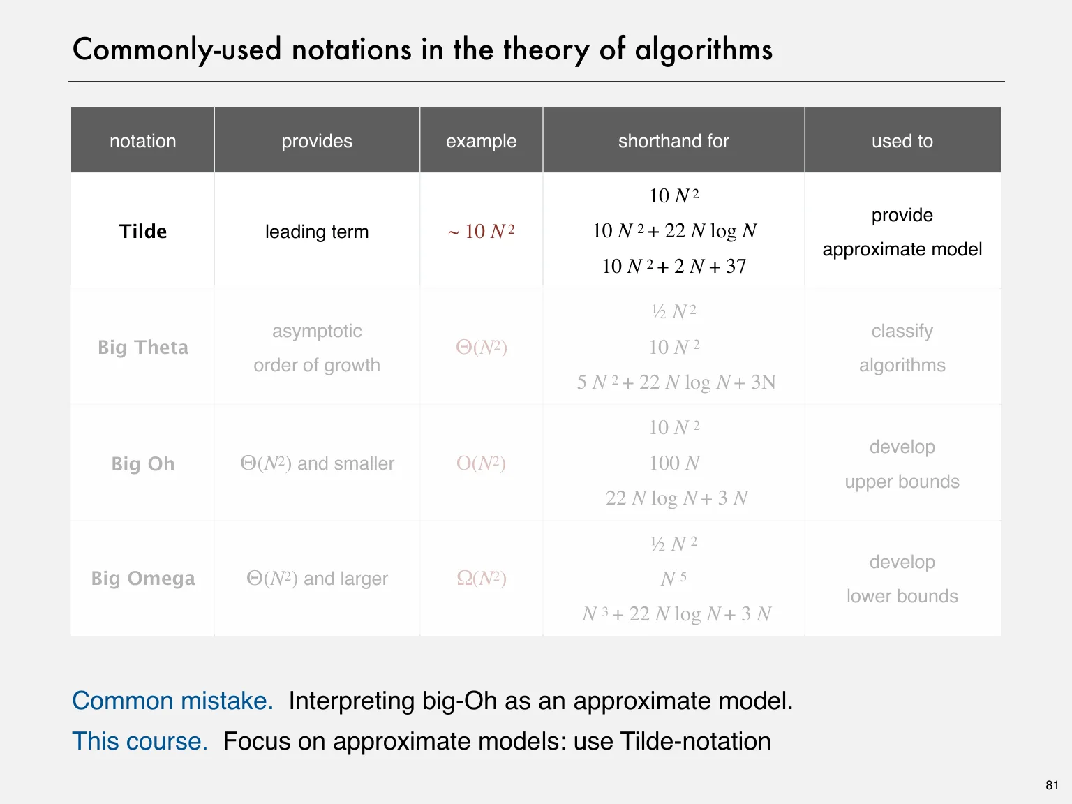
Distinguish tilde approximation from asymptotic bounds.
Analyze binary search and the faster 3-SUM approach.
Before you begin: Loops and arrays · Logarithms · Basic summations
Expanded study guide
Observe, model, predict, validate
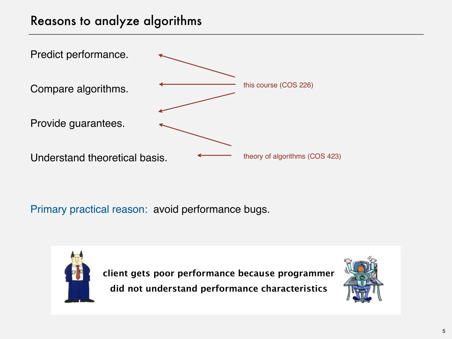
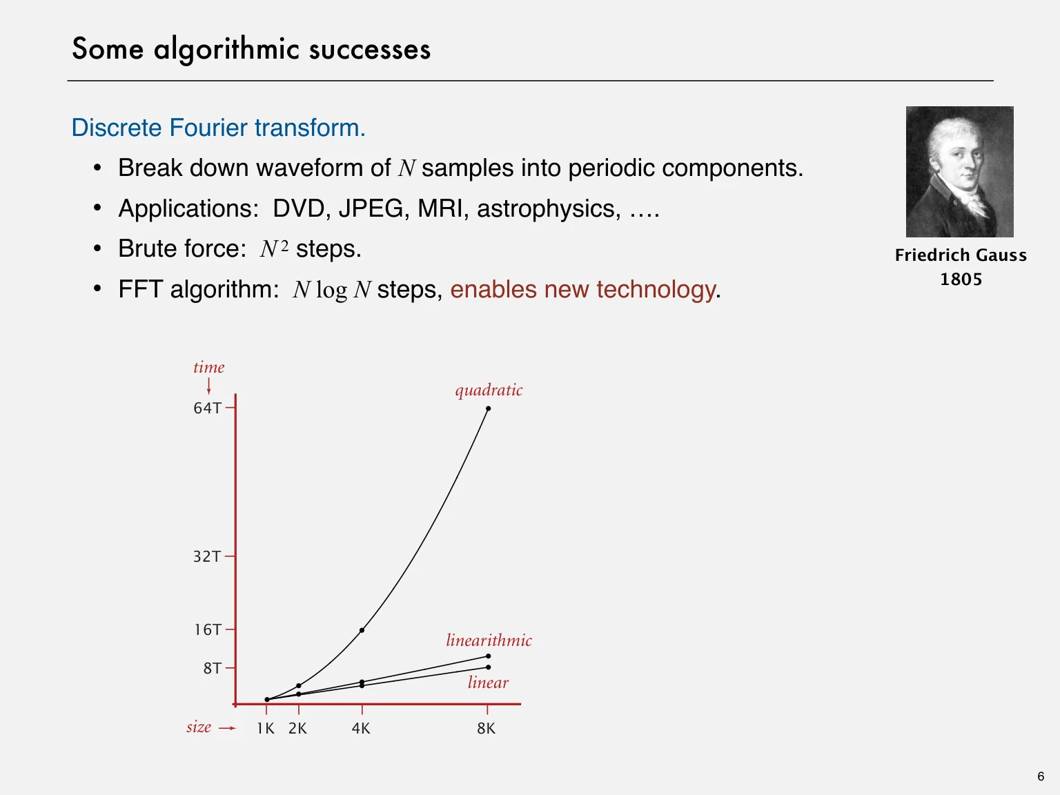
Algorithm analysis helps predict performance, compare alternatives, provide guarantees and avoid performance bugs. The source contrasts improvements such as a quadratic Fourier transform with a linearithmic FFT to show why growth matters.
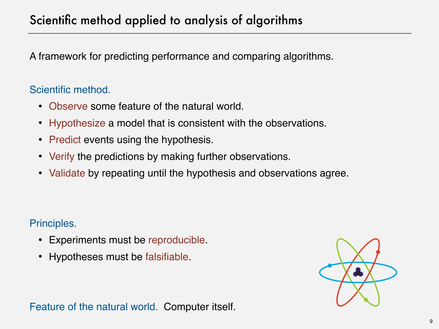
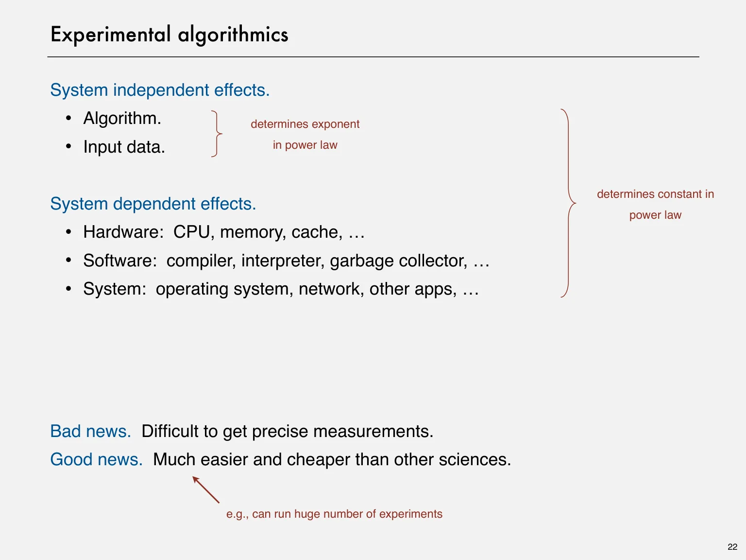
Measure a program on several input sizes, propose a model, predict a larger run, and compare the prediction with a fresh observation. A model should be reproducible and falsifiable. Hardware, runtime compilation, garbage collection and other activity can affect measurements.
3-SUM: count the work
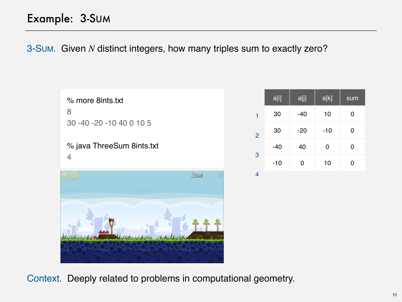
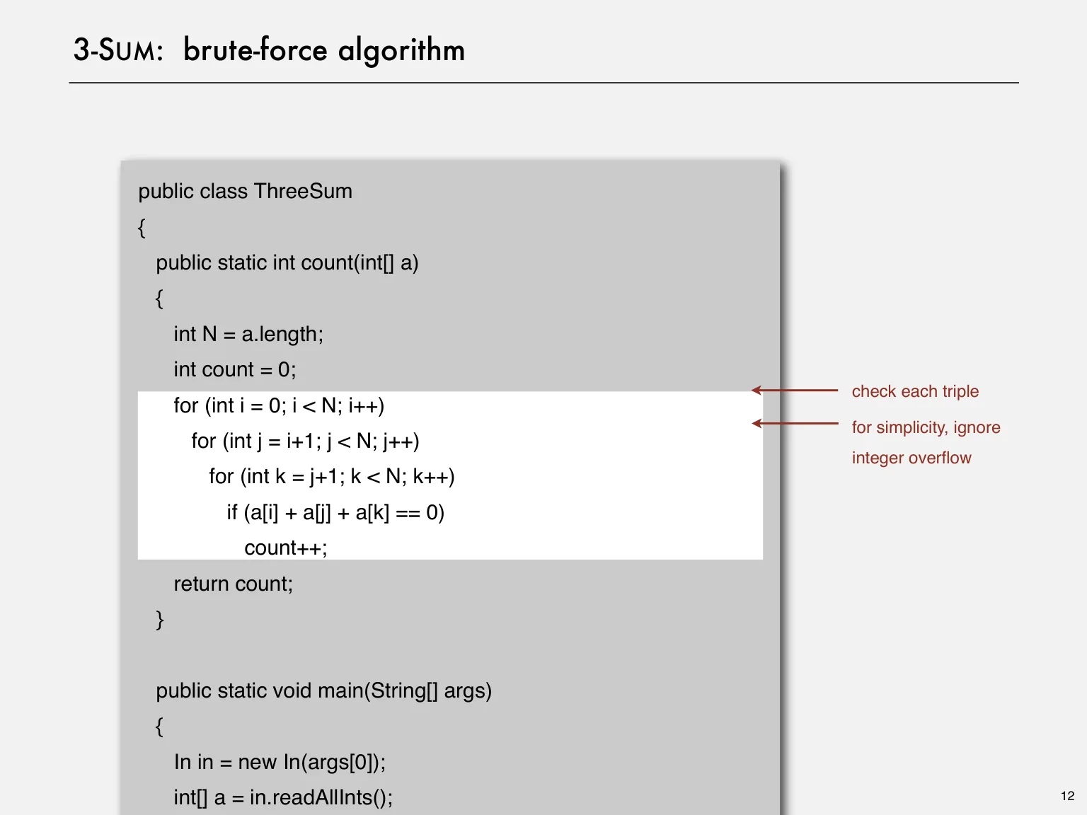
The source problem asks how many triples of distinct input integers sum to zero. The brute-force implementation iterates over indices i < j < k. This prevents counting the same triple in different orders.
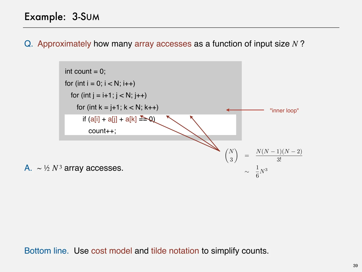
Every triple is tested regardless of whether a zero sum is found. There are n choose 3 triples, giving Θ(n³) tests. The count is not n³ exactly: the dependent loop bounds matter.
(3n)=6n(n−1)(n−2)∼6n3
Doubling experiments
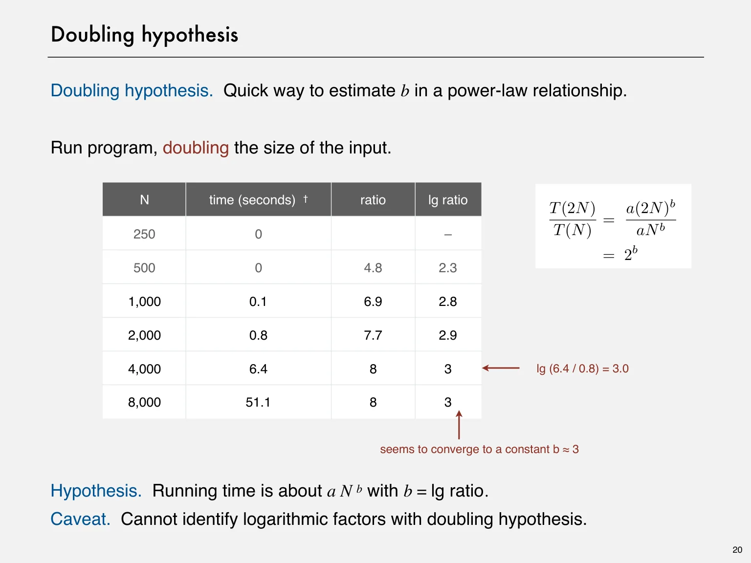
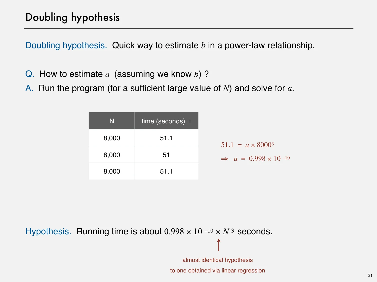
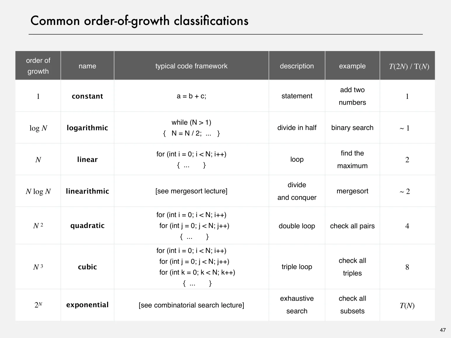
If T(n) ≈ anᵇ, then T(2n) / T(n) ≈ 2ᵇ. A ratio near 8 suggests cubic growth. Estimate b with the base-two logarithm of the ratio, then estimate a from a sufficiently large measurement.
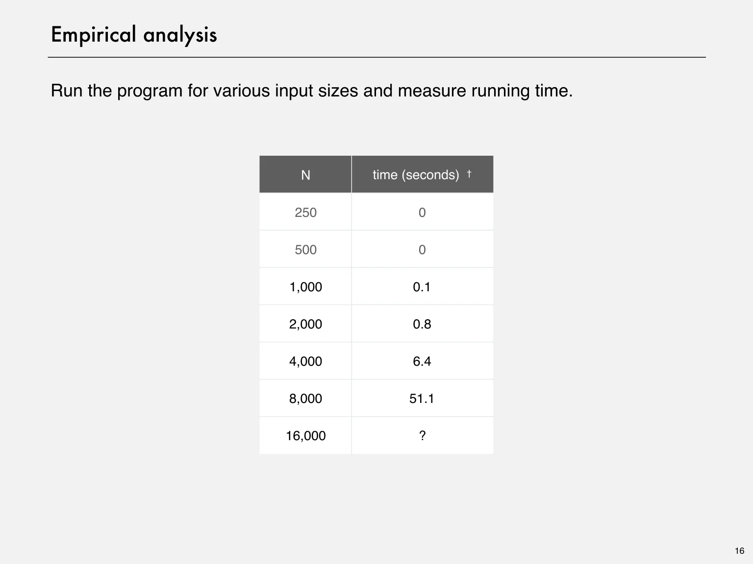
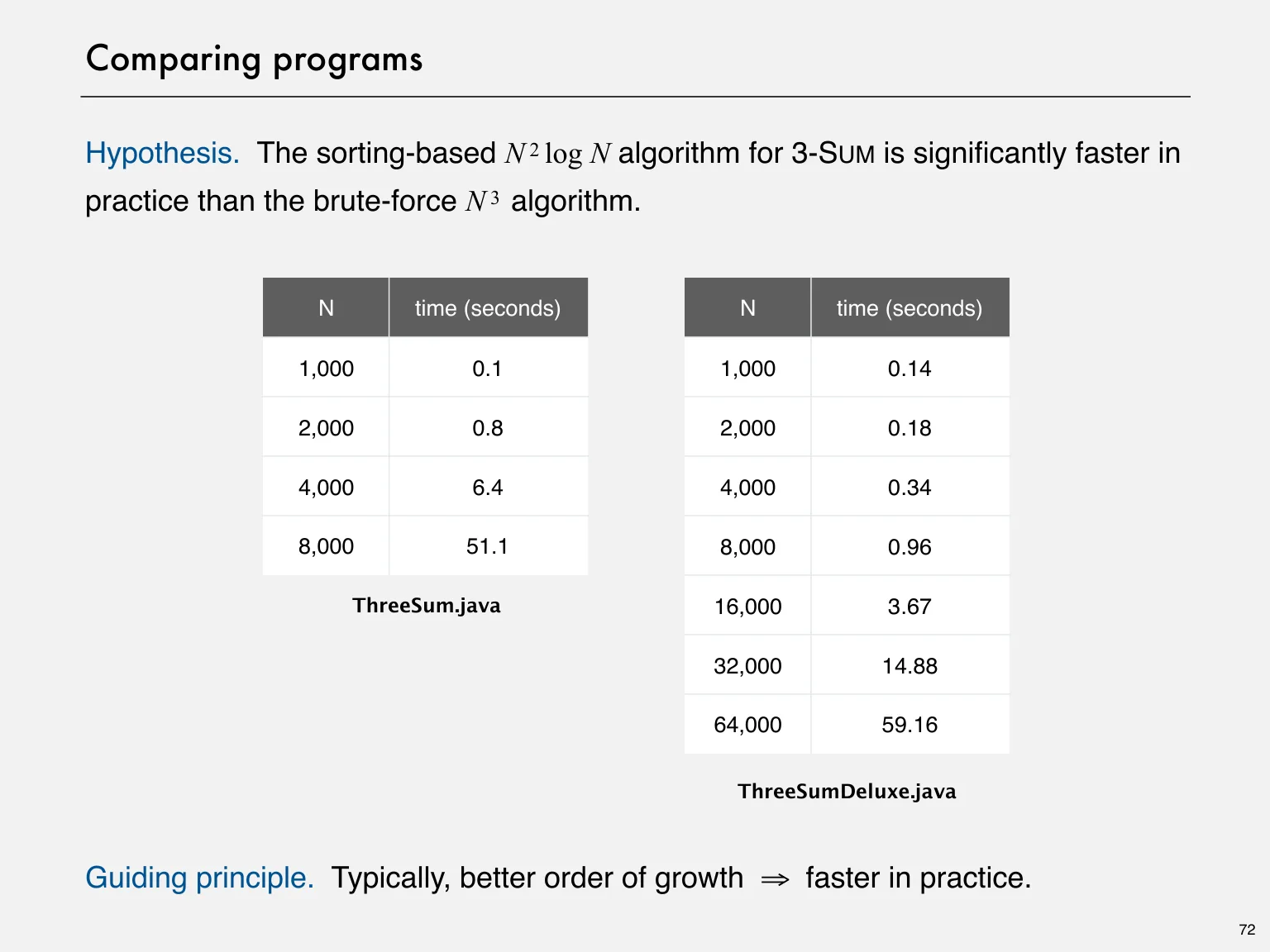
The source timing table gives about 0.1, 0.8, 6.4 and 51.1 seconds at successive doubled input sizes. These are historical observations, not promised timings on your device. Small measurements may be dominated by timer resolution or startup cost.
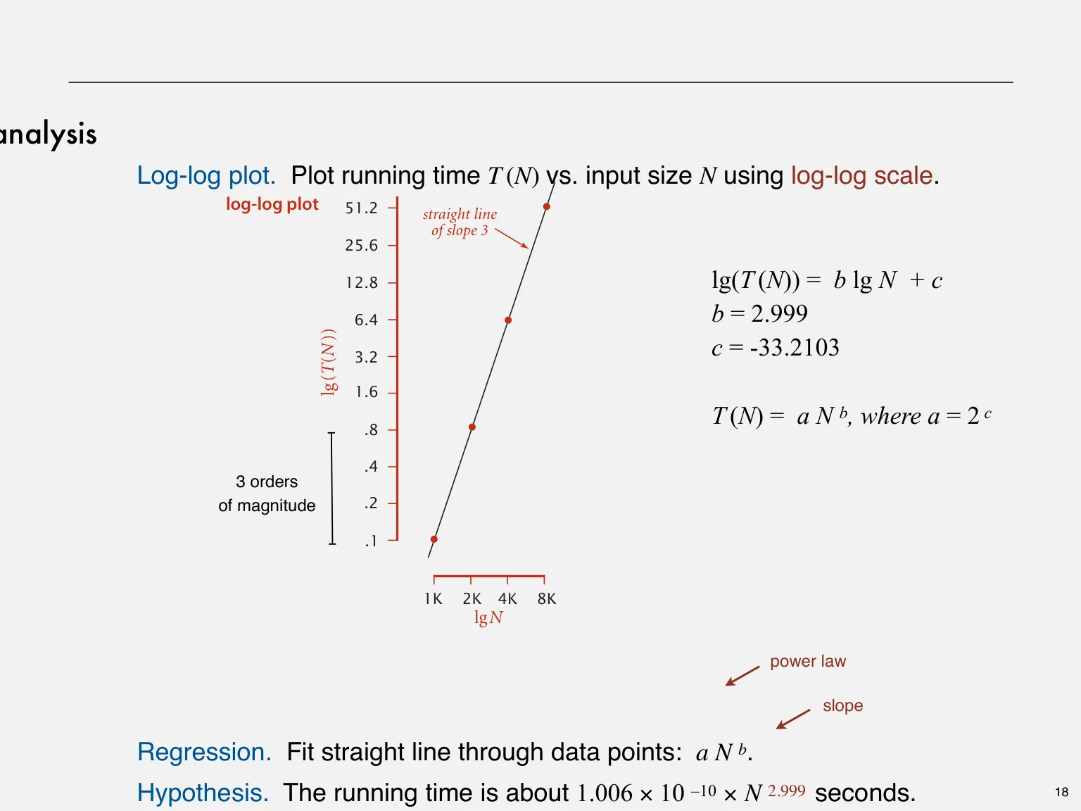
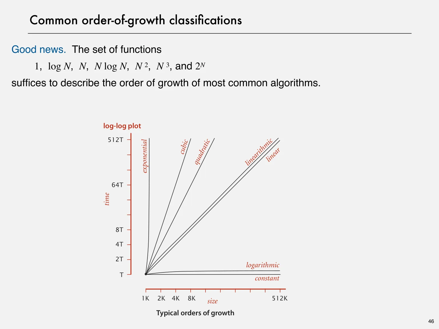
A doubling test does not prove a complexity result and can hide logarithmic factors. A log-log plot turns a power-law model into a line whose slope estimates the exponent.
b≈log2(T(n)T(2n)),T(n)≈anb
Cost models and finite sums
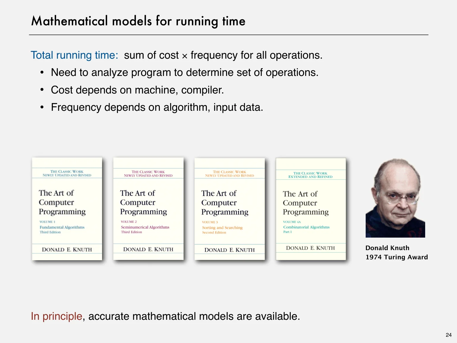
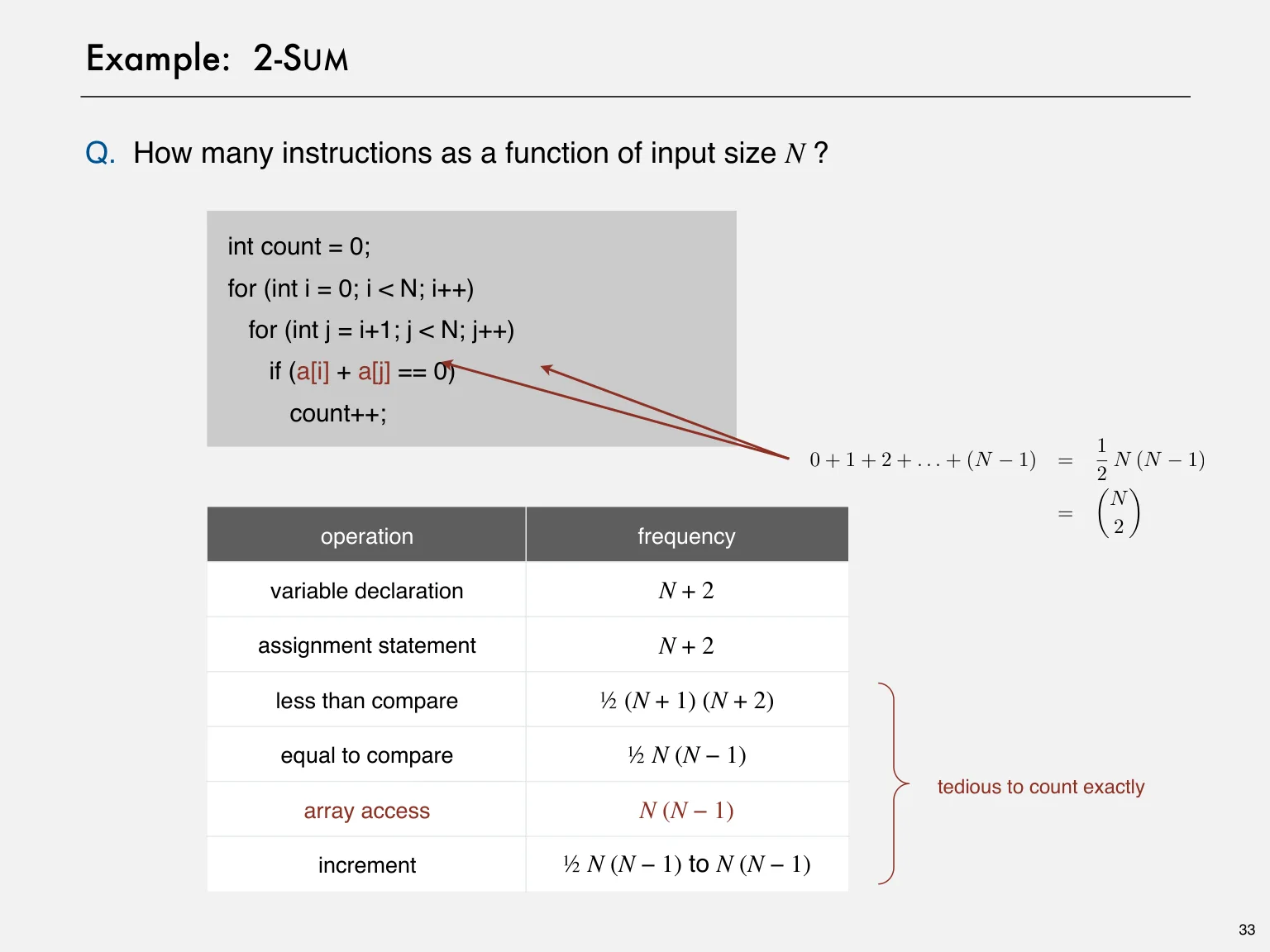
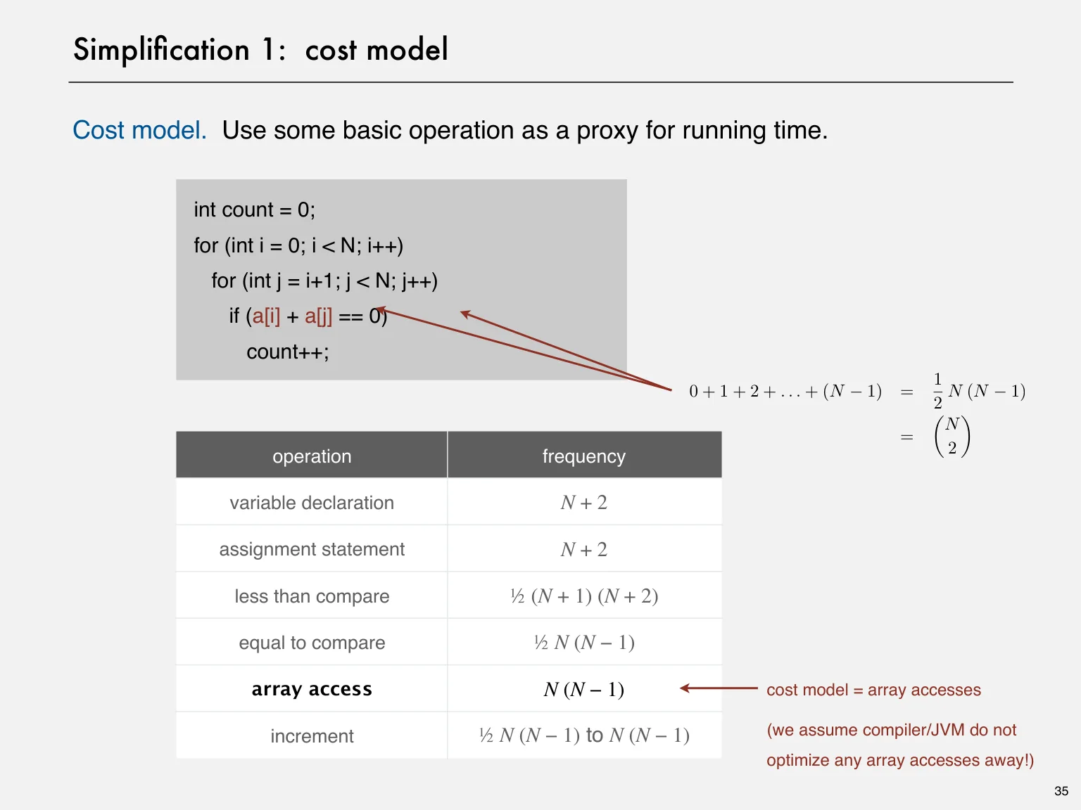
Total running time is modelled as the sum of each operation’s cost multiplied by its execution frequency. A cost model chooses an operation, such as an array access or key comparison, as a useful proxy.
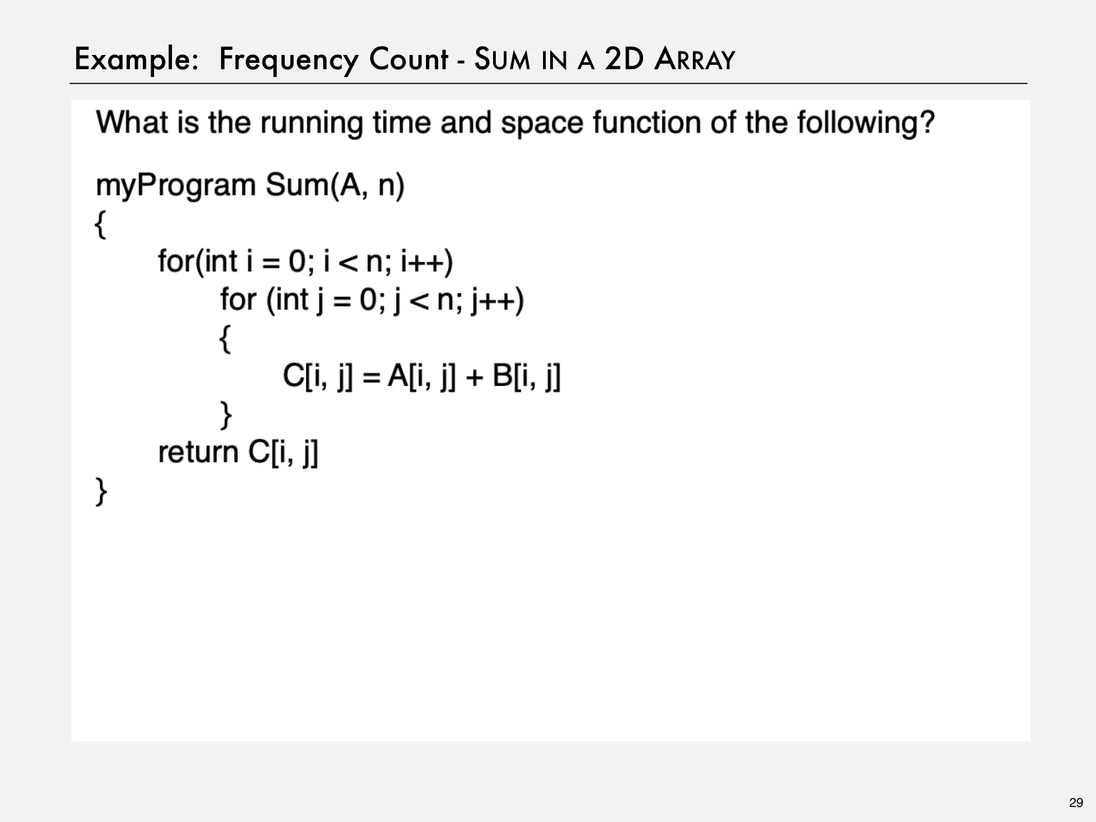
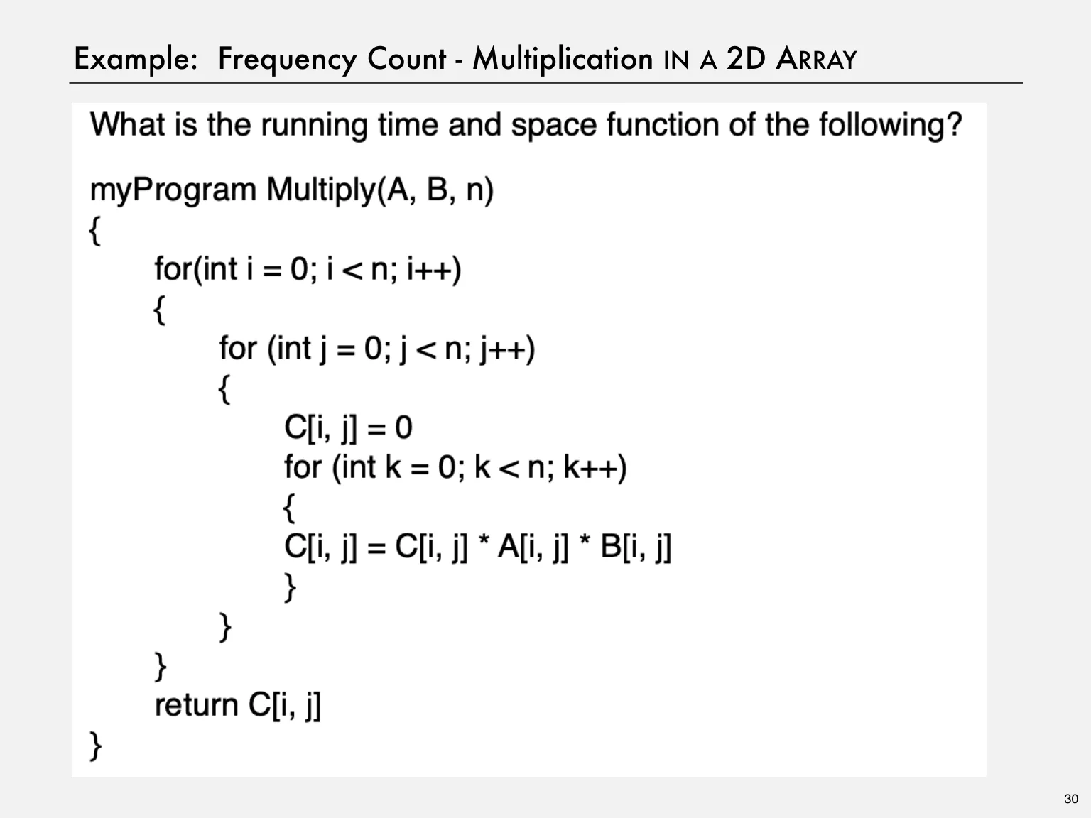
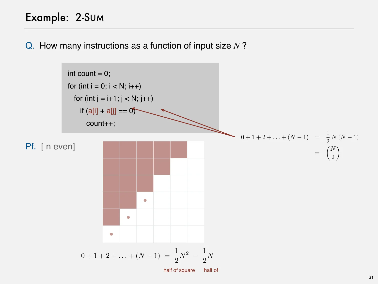
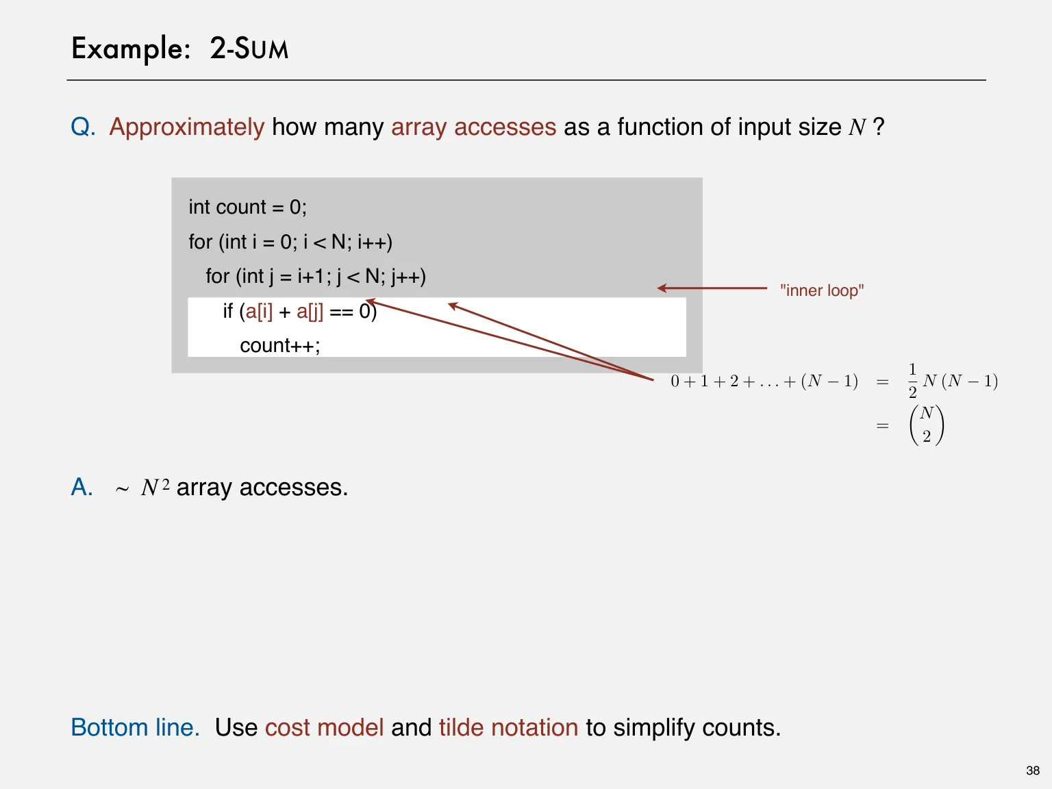
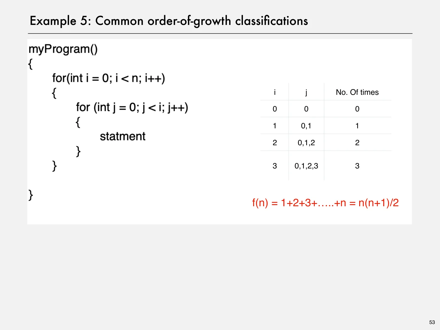
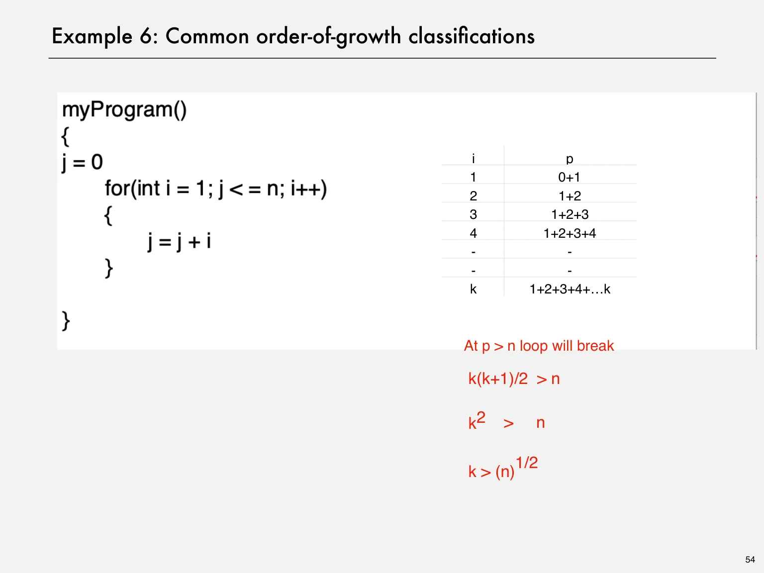
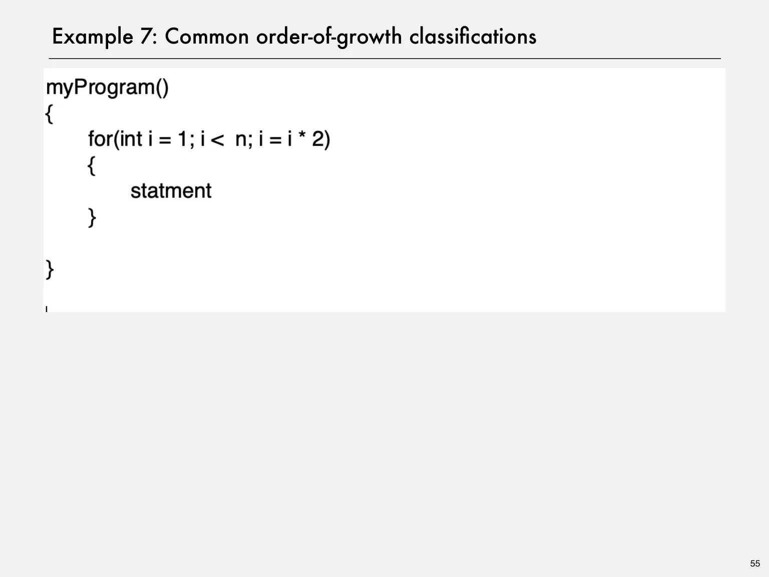
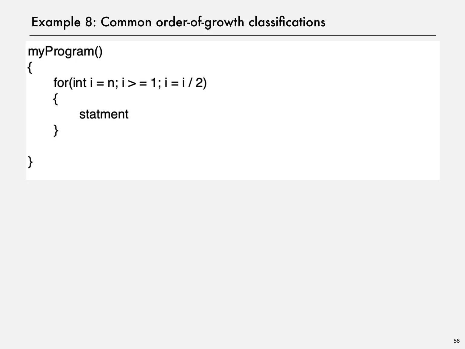
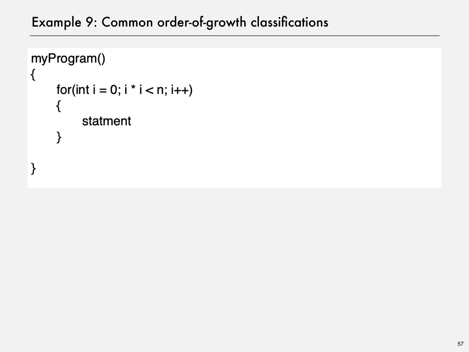
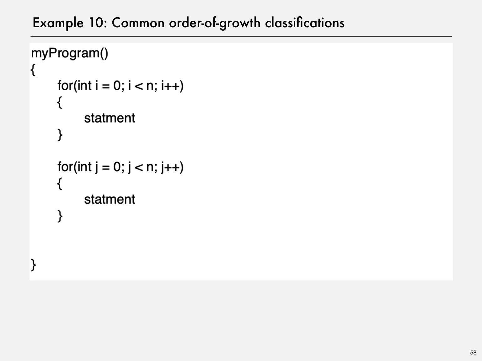
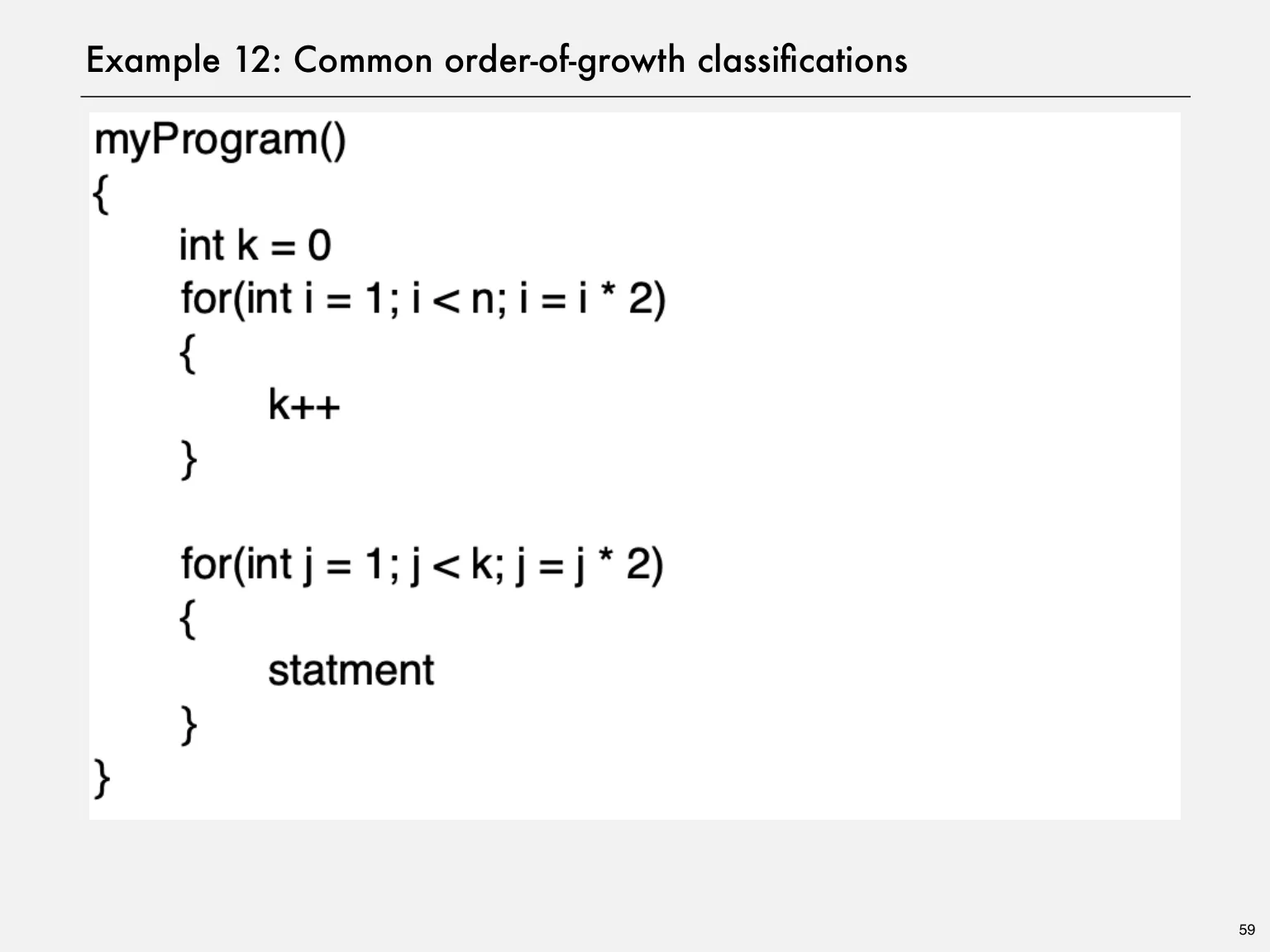
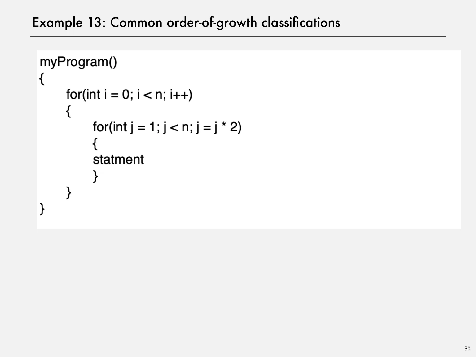
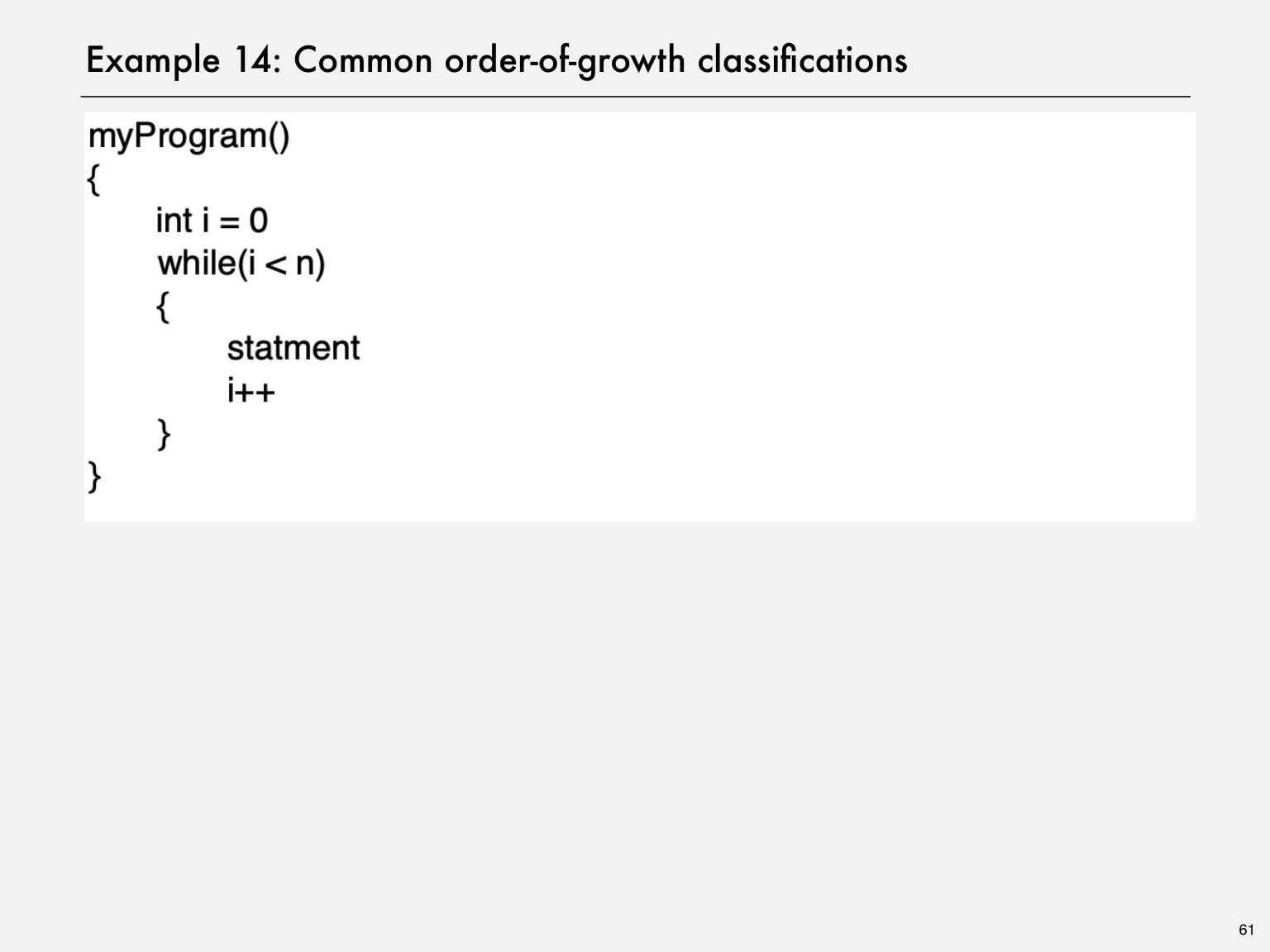
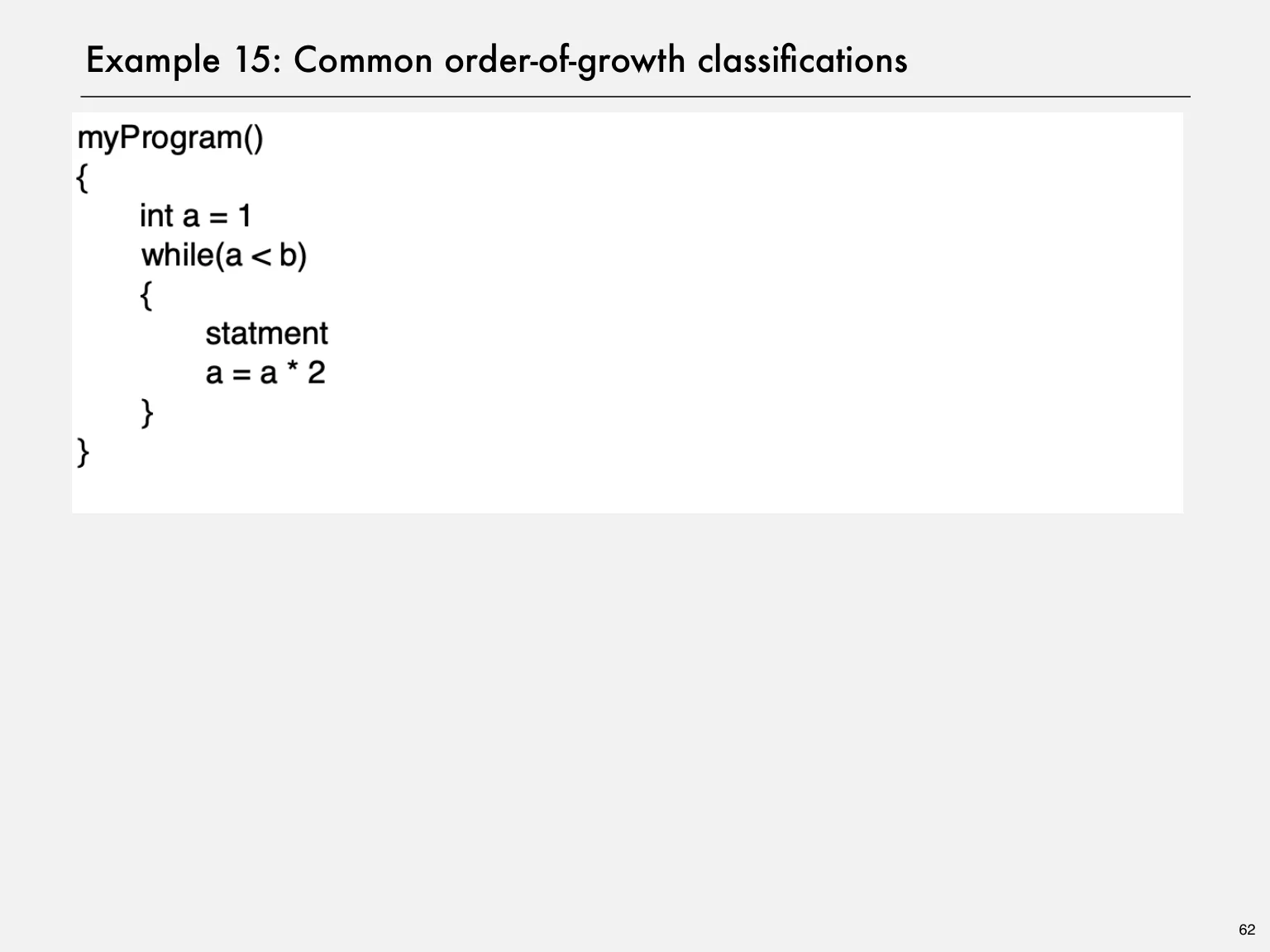
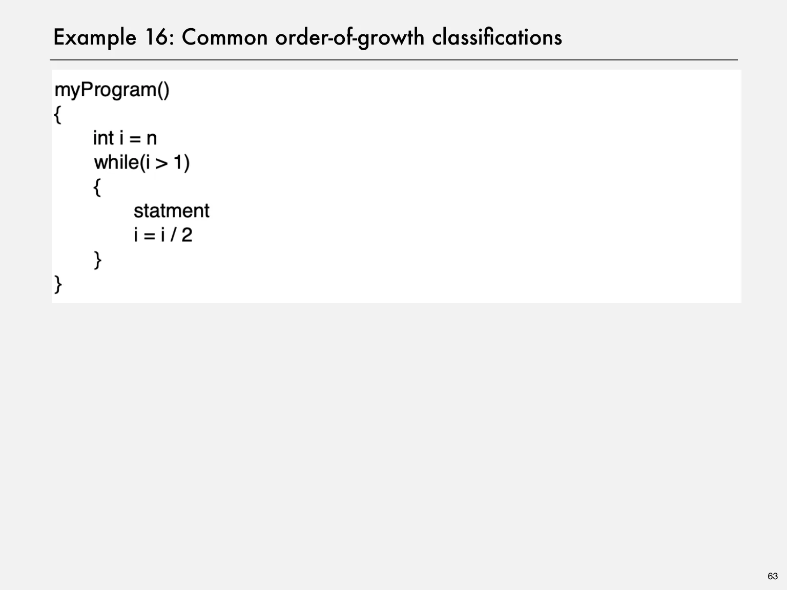
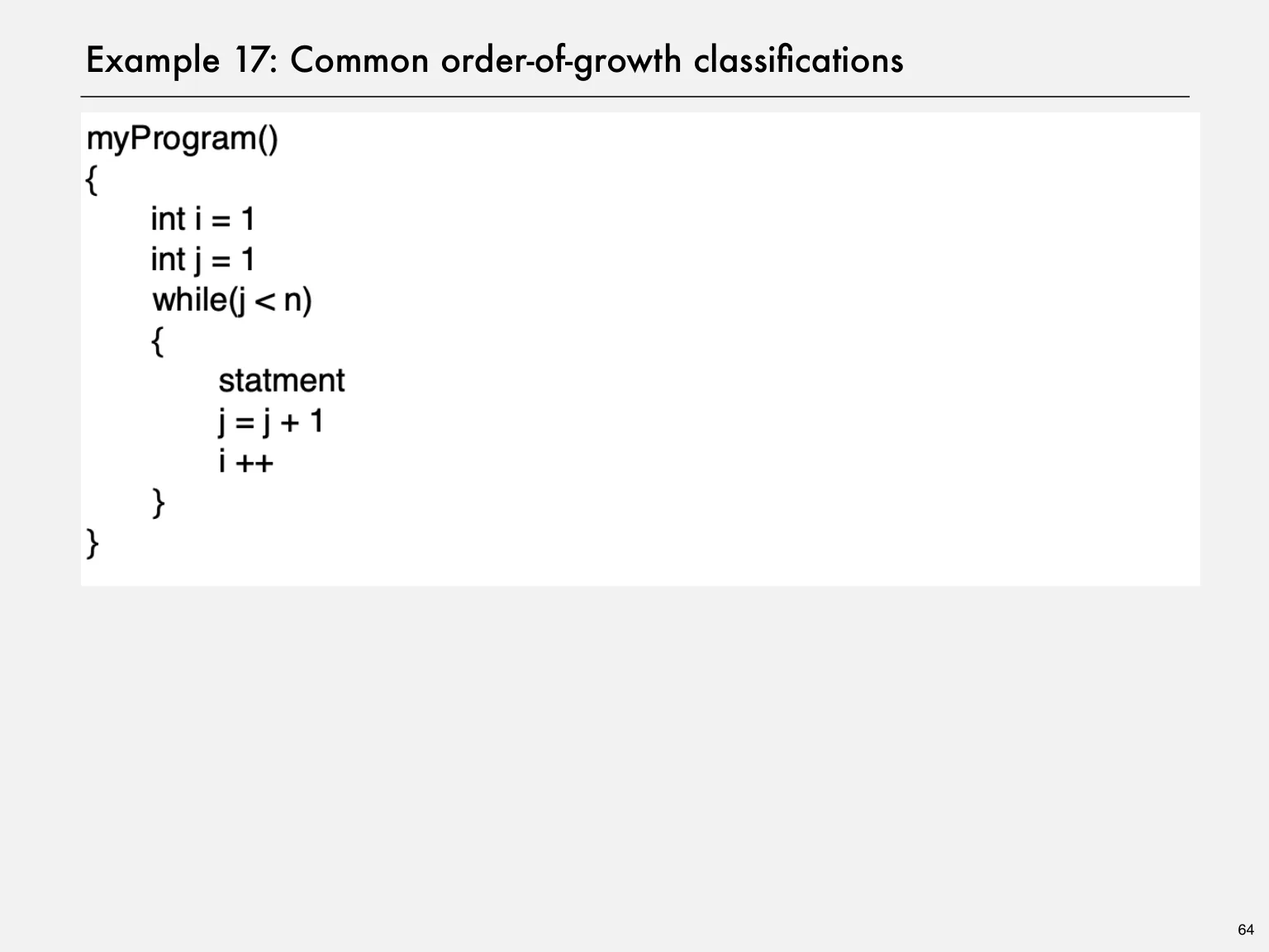
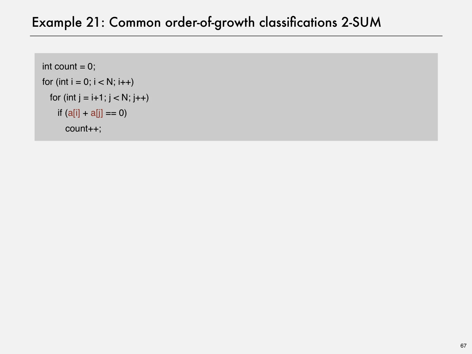
A scan performs Θ(n) work. Testing all pairs i < j performs n(n−1)/2 tests. A rectangular nested loop with n iterations in each level performs n² inner operations. A loop that repeatedly halves a counter performs Θ(log n) iterations.
Sequential blocks add their costs; nested blocks require summing the inner cost over the outer iterations.
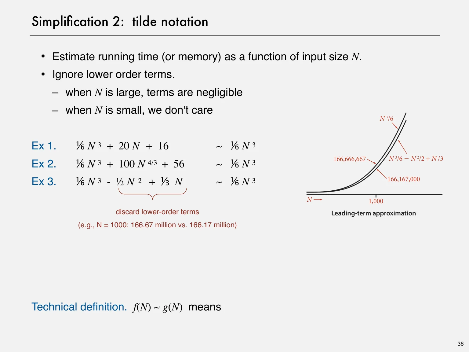
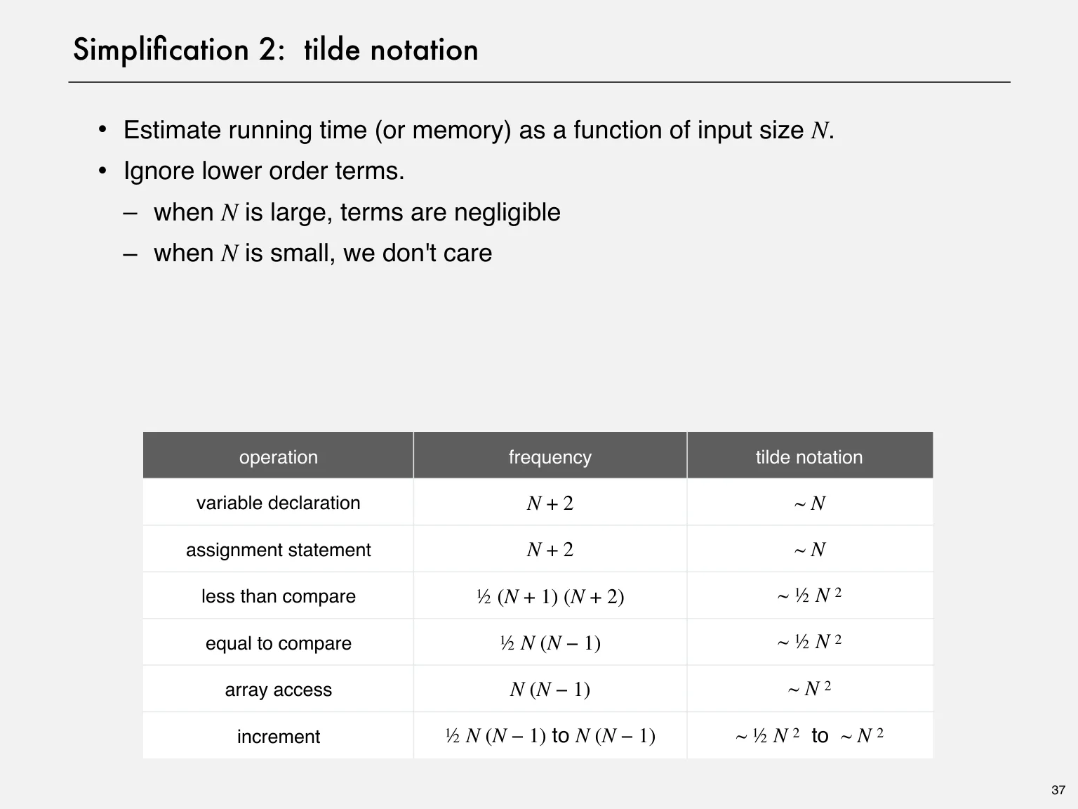
Tilde notation f(n) ~ g(n) means their ratio tends to 1, so the leading coefficient is retained.
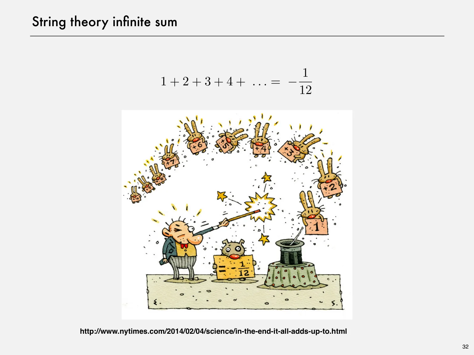
Slide 32’s 1 + 2 + 3 + … = −1/12 is a regularization diversion, not an ordinary convergent sum. Finite operation counts use ordinary finite sums.
i=0∑n−1i=2n(n−1),i=0∑k2i=2k+1−1
Binary search and its invariant
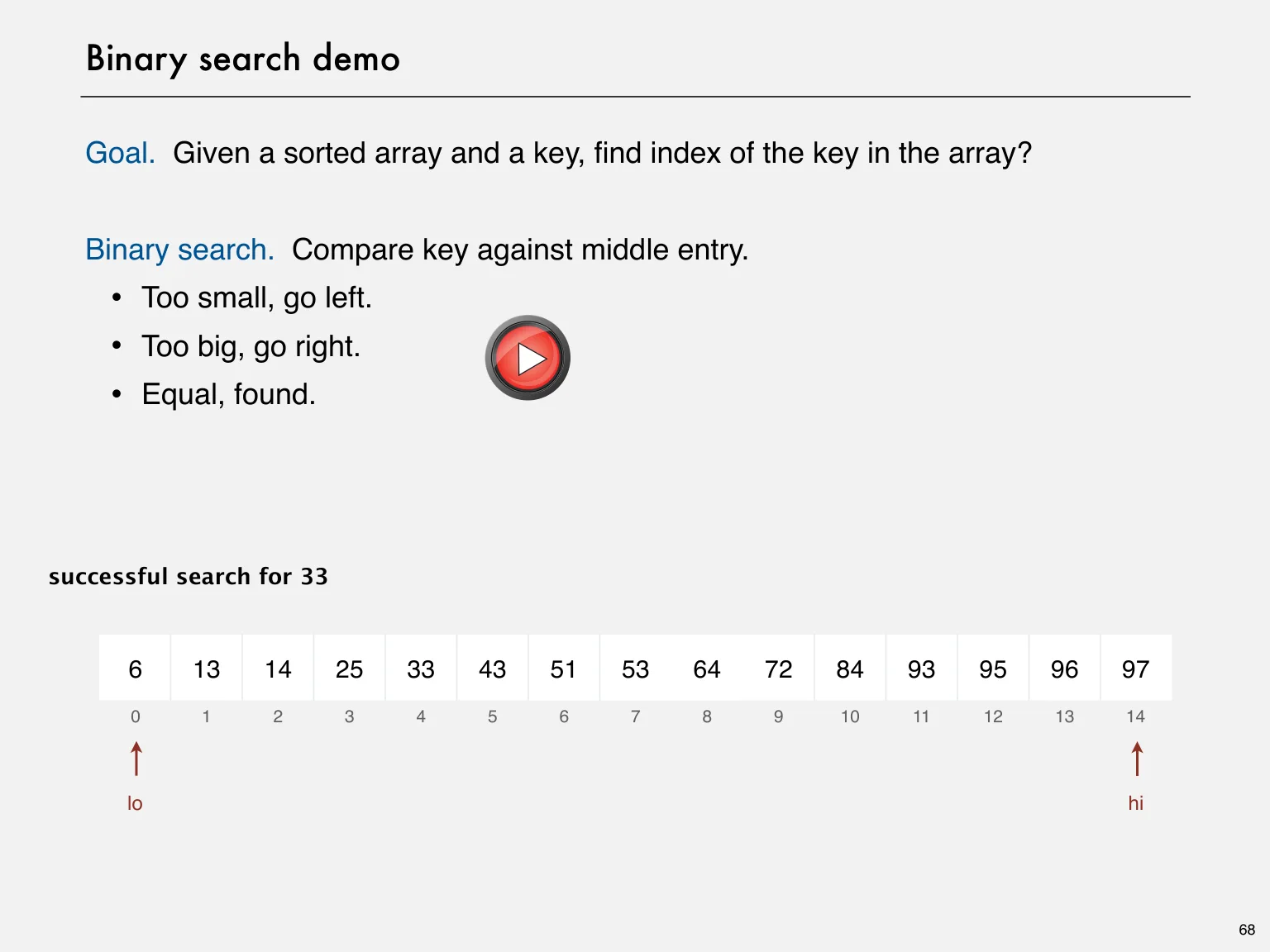
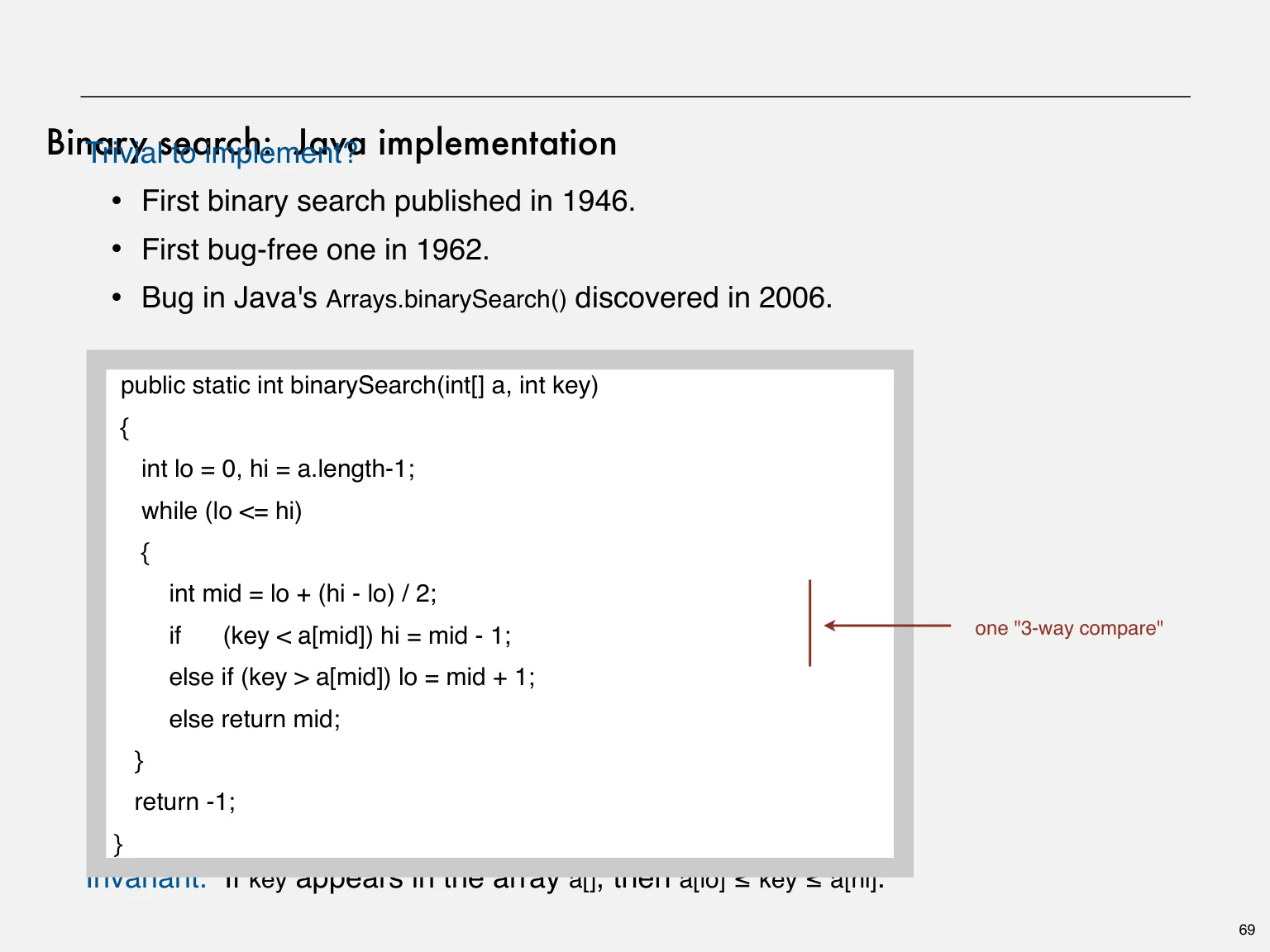
Binary search keeps an inclusive interval [lo, hi] in a sorted array. Compare the key with the middle element. Move hi left if the key is smaller, or move lo right if the key is larger. Equality returns the index. An empty interval proves absence.
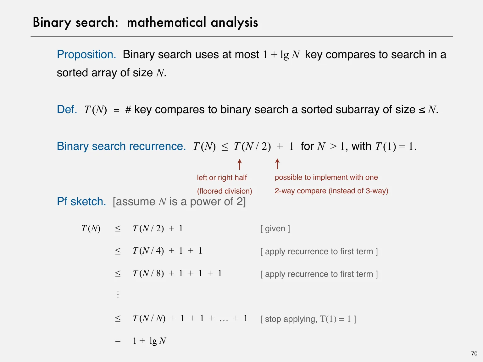
After k unsuccessful steps the candidate region has size at most about n/2ᵏ. This gives at most floor(log₂ n) + 1 middle-element inspections for a nonempty array. The supplied implementation is iterative and needs only constant auxiliary space.
The Java code computes mid = lo + (hi − lo) / 2 to avoid adding two large bounds.
Use hi = mid − 1 or lo = mid + 1 so the interval strictly shrinks.
The precise number of primitive comparisons depends on how the three-way decision is implemented.
T(n)≤T(⌊n/2⌋)+O(1)=O(logn)
Interactive dry run
Follow the search interval
6131425334351
Step 1 of 2: 25 < 43: discard indices 0 through 3.
A faster 3-SUM strategy
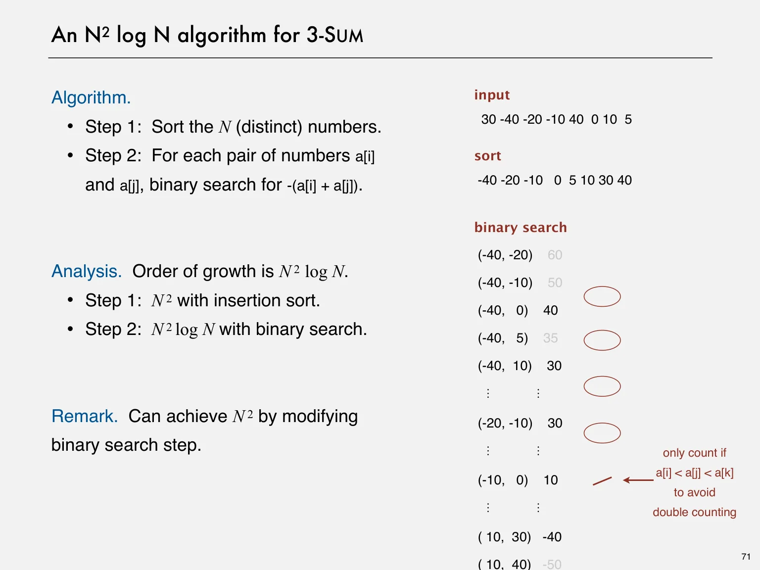
Sort the array. For each index pair i < j, binary-search for −(a[i] + a[j]). Count it only when the returned index is greater than j. The pair loops cost Θ(n²), and each search is O(log n), so the overall worst-case growth is O(n² log n), including a lower-order sorting step.
ThreeSumFast.java rejects duplicate input integers. Preserve that precondition when comparing results. Both integer addition and negation can overflow in Java; the original source’s arithmetic caveat should be considered when selecting test inputs.
Cases, bounds and optimality
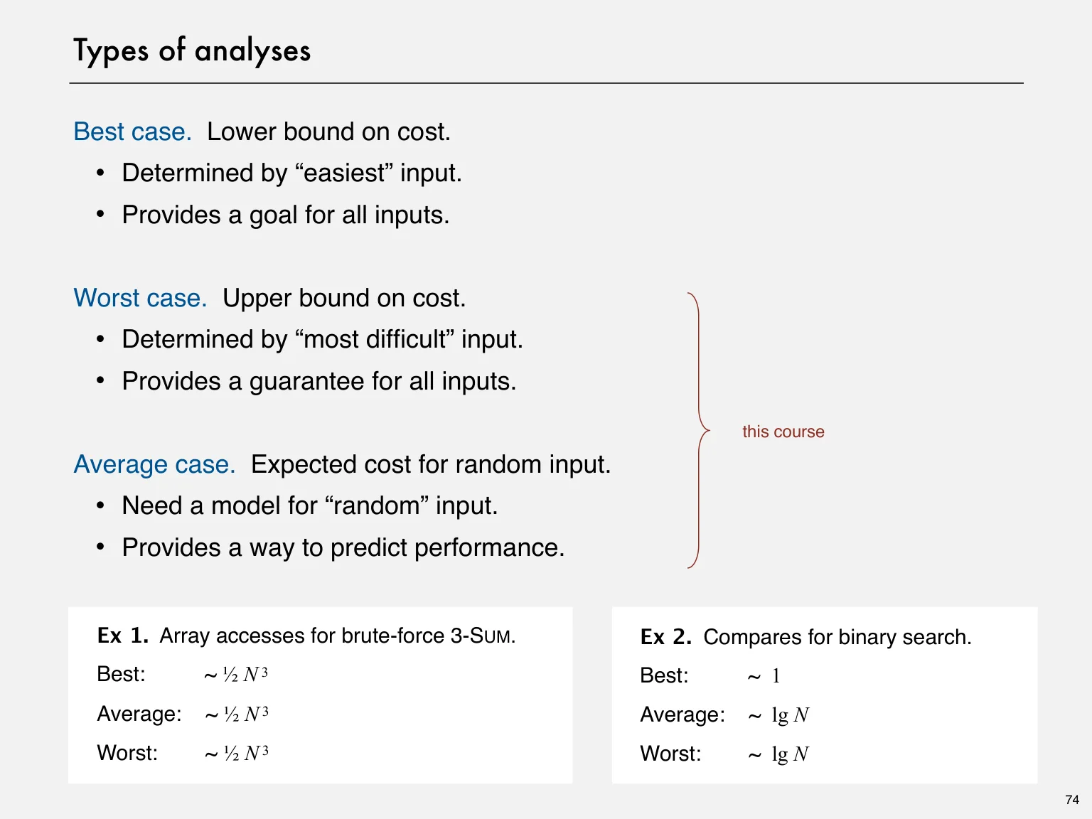
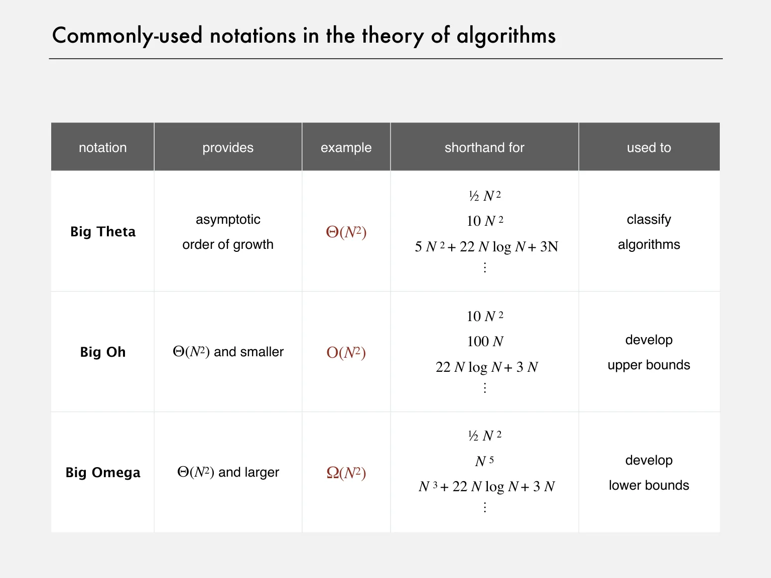
Best case minimizes cost over inputs of a fixed size. Worst case maximizes it. Average case takes an expectation under a specified input distribution. These choices describe the cost function; O, Ω and Θ describe bounds on that function.
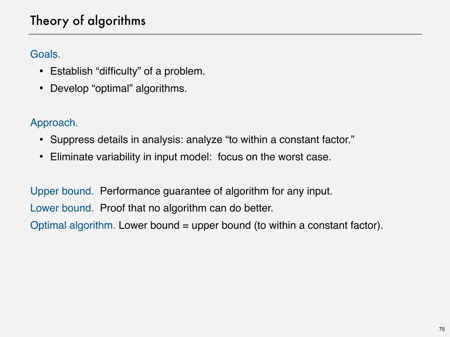
An algorithm provides an upper bound on a problem’s difficulty. A problem lower bound applies to every algorithm in the stated model. A matching upper and lower bound establishes asymptotic optimality in that model. Historical open-problem statements in the slides should not be treated as current research claims.
Space is a resource too
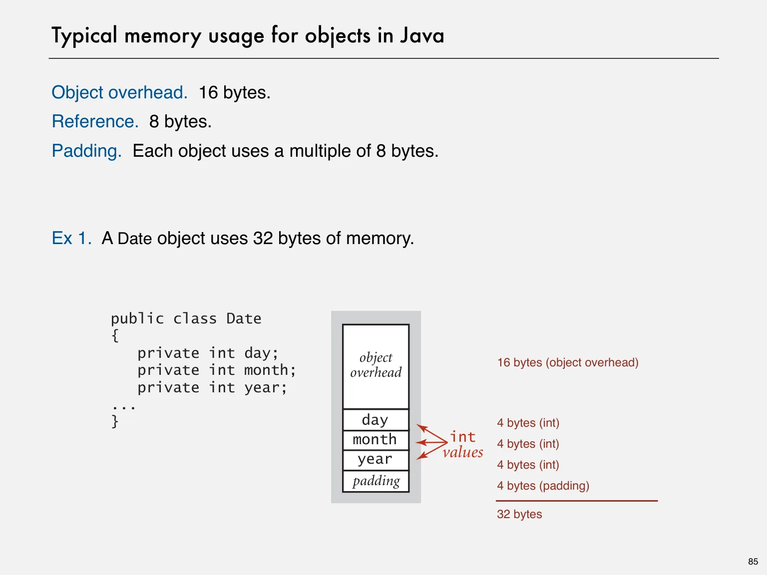
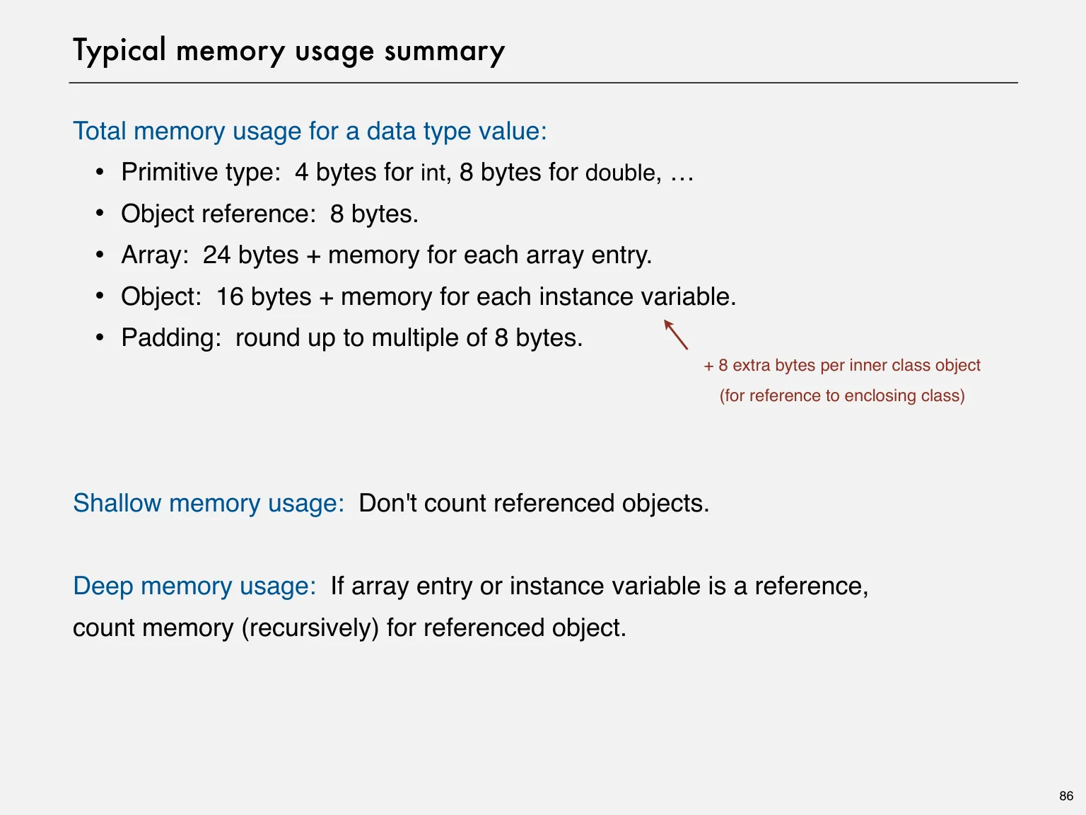
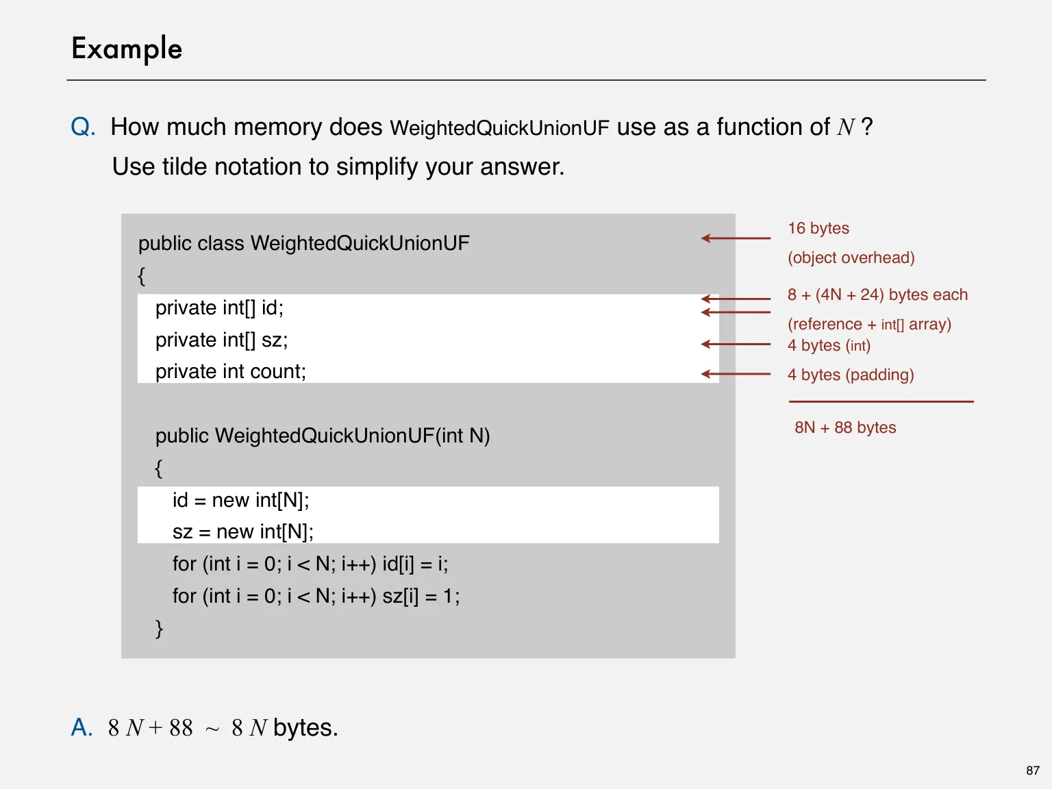
Count the input, arrays, objects, references and recursion frames deliberately. State whether you report total space or auxiliary space beyond the input. The source’s byte counts assume a particular 64-bit Java object model; headers, padding and reference sizes are implementation-dependent.
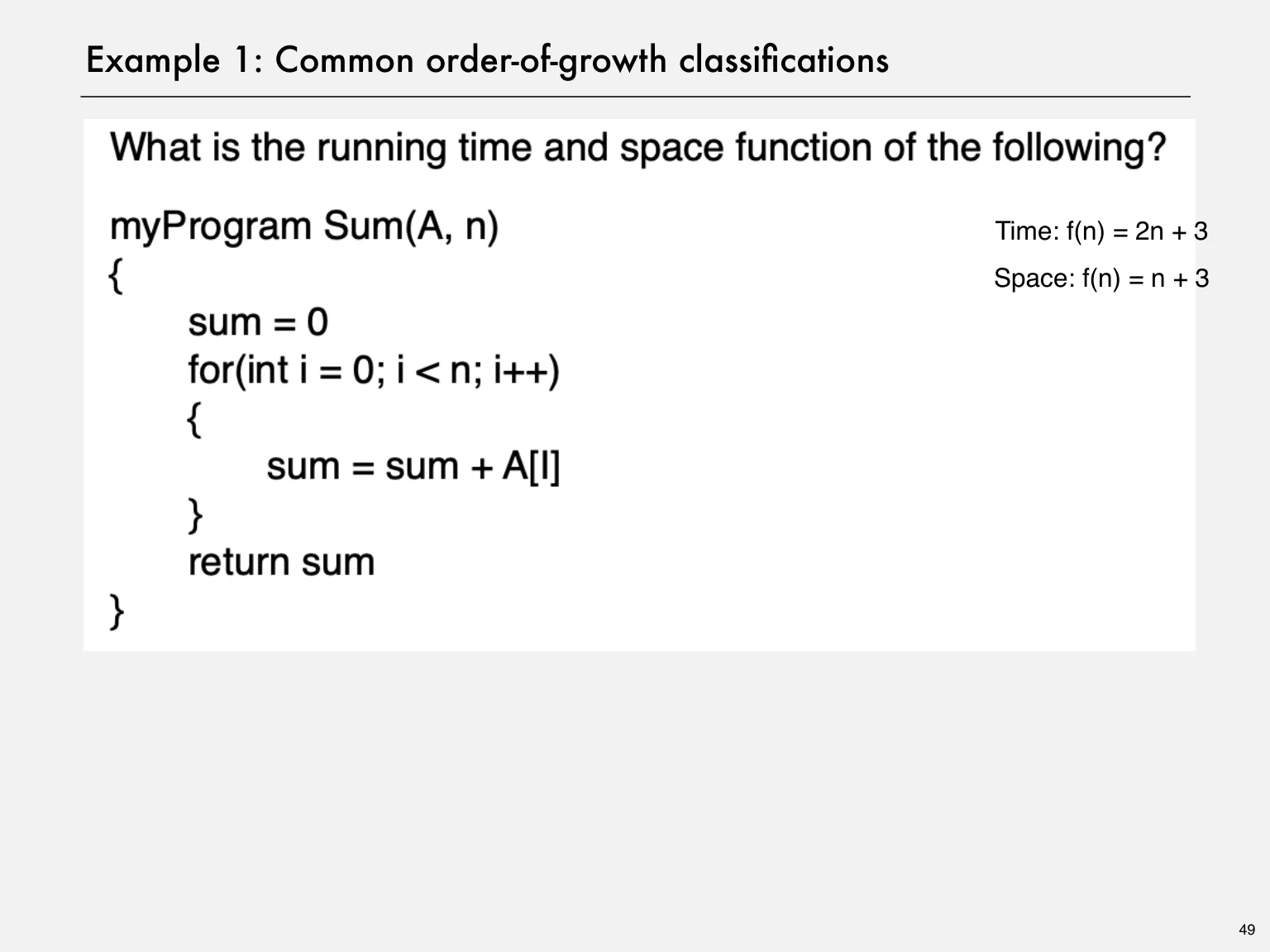
A nested loop does not automatically require quadratic space. ThreeSum uses a few counters beyond the input array despite cubic time. A recursive procedure can use stack memory even without explicitly allocating an array.
A useful analysis checklist
Define n and the input assumptions. Select a cost model. Count operations or derive a recurrence. Simplify with the appropriate notation. Separate empirical observations from proofs, and state the memory model.
Original implementations
Read the complete original code and its documentation. Core algorithm pages add a walkthrough, complexity discussion and a worked example.
Supplementary practice. Try each question before opening the answer.
A run takes 2 seconds at n and 16 seconds at 2n. What exponent does the doubling hypothesis suggest?
The ratio is 8, so b = log₂8 = 3. This suggests a cubic power law, but more measurements and a mathematical argument are needed.
Why is 3-SUM’s triple count n(n−1)(n−2)/6?
Each unordered selection of three distinct indices is visited exactly once because i < j < k. Dividing ordered selections by 3! gives the count.
Does Θ(n³) running time imply Θ(n³) memory?
No. Time counts work; space counts simultaneously stored data. The brute-force 3-SUM loop uses constant auxiliary space.
Original course material
Complete lecture source
Every source page is preserved below. Open a page to read its text and inspect the original diagram, formula or example. Expanded explanations above are supplementary.
Page 01 · ROBERT SEDGEWICK | KEVIN WAYNE AlgorithmsOriginal page 1 · Open the image for full detail.
ROBERT SEDGEWICK | KEVIN WAYNE Algorithms
1.4 ANALYSIS OF
‣ introduction
‣ observations
‣ mathematical models
AlgorithmsF O U R T H E D I T I O N
‣ order-of-growth classifications
‣ theory of algorithms
ROBERT SEDGEWICK | KEVIN WAYNE
http://algs4.cs.princeton.edu ‣ memory
Page 02 · 1.4 ANALYSIS OFOriginal page 2 · Open the image for full detail.
1.4 ANALYSIS OF
‣ introduction
‣ observations
‣ mathematical modelsAlgorithms
‣ order-of-growth classifications
‣ theory of algorithms
ROBERT SEDGEWICK | KEVIN WAYNE
http://algs4.cs.princeton.edu ‣ memory
Page 03 · Running timeOriginal page 3 · Open the image for full detail.
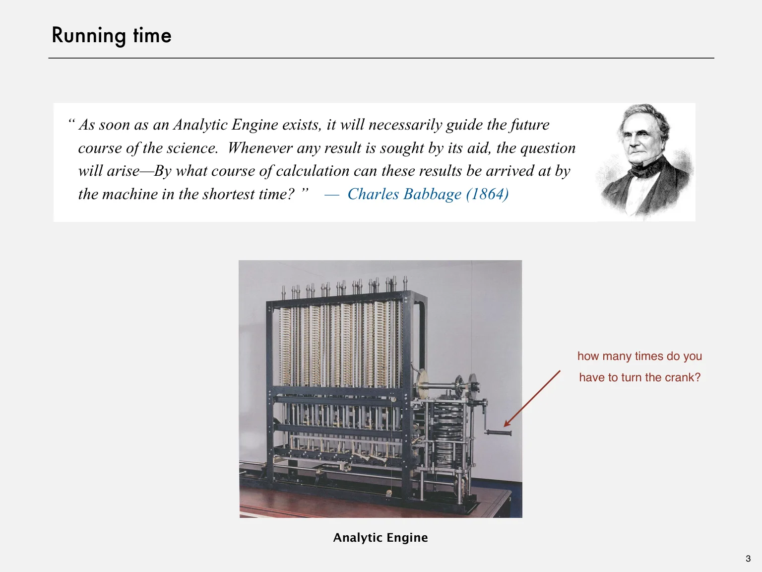
Running time
“ As soon as an Analytic Engine exists, it will necessarily guide the future
course of the science. Whenever any result is sought by its aid, the question
will arise—By what course of calculation can these results be arrived at by
the machine in the shortest time? ” — Charles Babbage (1864)
how many times do you
have to turn the crank?
Analytic Engine
3
Page 04 · Cast of charactersOriginal page 4 · Open the image for full detail.
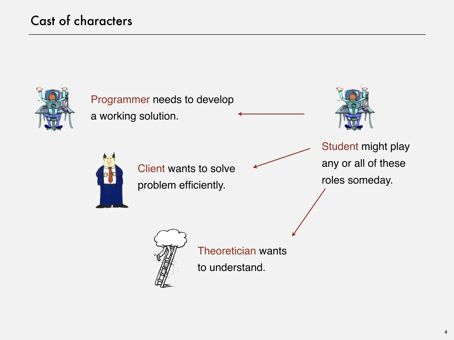
Cast of characters
Programmer needs to develop
a working solution.
Student might play
any or all of these Client wants to solve
roles someday. problem efficiently.
Theoretician wants
to understand.
4
Page 05 · Reasons to analyze algorithmsOriginal page 5 · Open the image for full detail.
Reasons to analyze algorithms
Predict performance.
this course (COS 226)
Compare algorithms.
Provide guarantees.
Understand theoretical basis. theory of algorithms (COS 423)
Primary practical reason: avoid performance bugs.
client gets poor performance because programmer
did not understand performance characteristics
5
Page 06 · Some algorithmic successesOriginal page 6 · Open the image for full detail.
Some algorithmic successes
Discrete Fourier transform.
down waveform of N samples into periodic components.・Break
DVD, JPEG, MRI, astrophysics, ….・Applications:
force: N 2 steps. Friedrich Gauss・Brute
1805
algorithm: N log N steps, enables new technology.・FFT
time
quadratic
64T
32T
16T
linearithmic
8T
linear
size 1K 2K 4K 8K
6
Page 07 · Some algorithmic successesOriginal page 7 · Open the image for full detail.
Some algorithmic successes
N-body simulation.
gravitational interactions among N bodies.・Simulate
force: N 2 steps.・Brute
algorithm: N log N steps, enables new research. Andrew Appel ・Barnes-Hut
PU '81
time
quadratic
64T
32T
16T
linearithmic
8T
linear
size 1K 2K 4K 8K
7
Page 08 · The challengeOriginal page 8 · Open the image for full detail.
The challenge
Q. Will my program be able to solve a large practical input?
Why is my program so slow ? Why does it run out of memory ?
Insight. [Knuth 1970s] Use scientific method to understand performance.
8
Page 09 · Scientific method applied to analysis of algorithmsOriginal page 9 · Open the image for full detail.
Scientific method applied to analysis of algorithms
A framework for predicting performance and comparing algorithms.
Scientific method.
some feature of the natural world.・Observe
a model that is consistent with the observations.・Hypothesize
events using the hypothesis.・Predict
the predictions by making further observations.・Verify
by repeating until the hypothesis and observations agree.・Validate
Principles.
must be reproducible.・Experiments
must be falsifiable.・Hypotheses
Feature of the natural world. Computer itself.
9
Page 10 · 1.4 ANALYSIS OFOriginal page 10 · Open the image for full detail.
1.4 ANALYSIS OF
‣ introduction
‣ observations
‣ mathematical modelsAlgorithms
‣ order-of-growth classifications
‣ theory of algorithms
ROBERT SEDGEWICK | KEVIN WAYNE
http://algs4.cs.princeton.edu ‣ memory
Page 11 · Example: 3-SUMOriginal page 11 · Open the image for full detail.
Example: 3-SUM
3-SUM. Given N distinct integers, how many triples sum to exactly zero?
a[i] a[j] a[k] sum % more 8ints.txt
8 30 -40 10 0 1
30 -40 -20 -10 40 0 10 5
30 -20 -10 0
2
% java ThreeSum 8ints.txt -40 40 0 0
3 4
-10 0 10 0
4
Context. Deeply related to problems in computational geometry.
11
Page 12 · 3-SUM: brute-force algorithmOriginal page 12 · Open the image for full detail.
3-SUM: brute-force algorithm
public class ThreeSum
{
public static int count(int[] a)
{
int N = a.length;
int count = 0;
check each triple
for (int i = 0; i < N; i++)
for simplicity, ignore
for (int j = i+1; j < N; j++)
integer overflow
for (int k = j+1; k < N; k++)
if (a[i] + a[j] + a[k] == 0)
count++;
return count;
}
public static void main(String[] args)
{
In in = new In(args[0]);
int[] a = in.readAllInts(); 12
Page 13 · Measuring the running timeOriginal page 13 · Open the image for full detail.
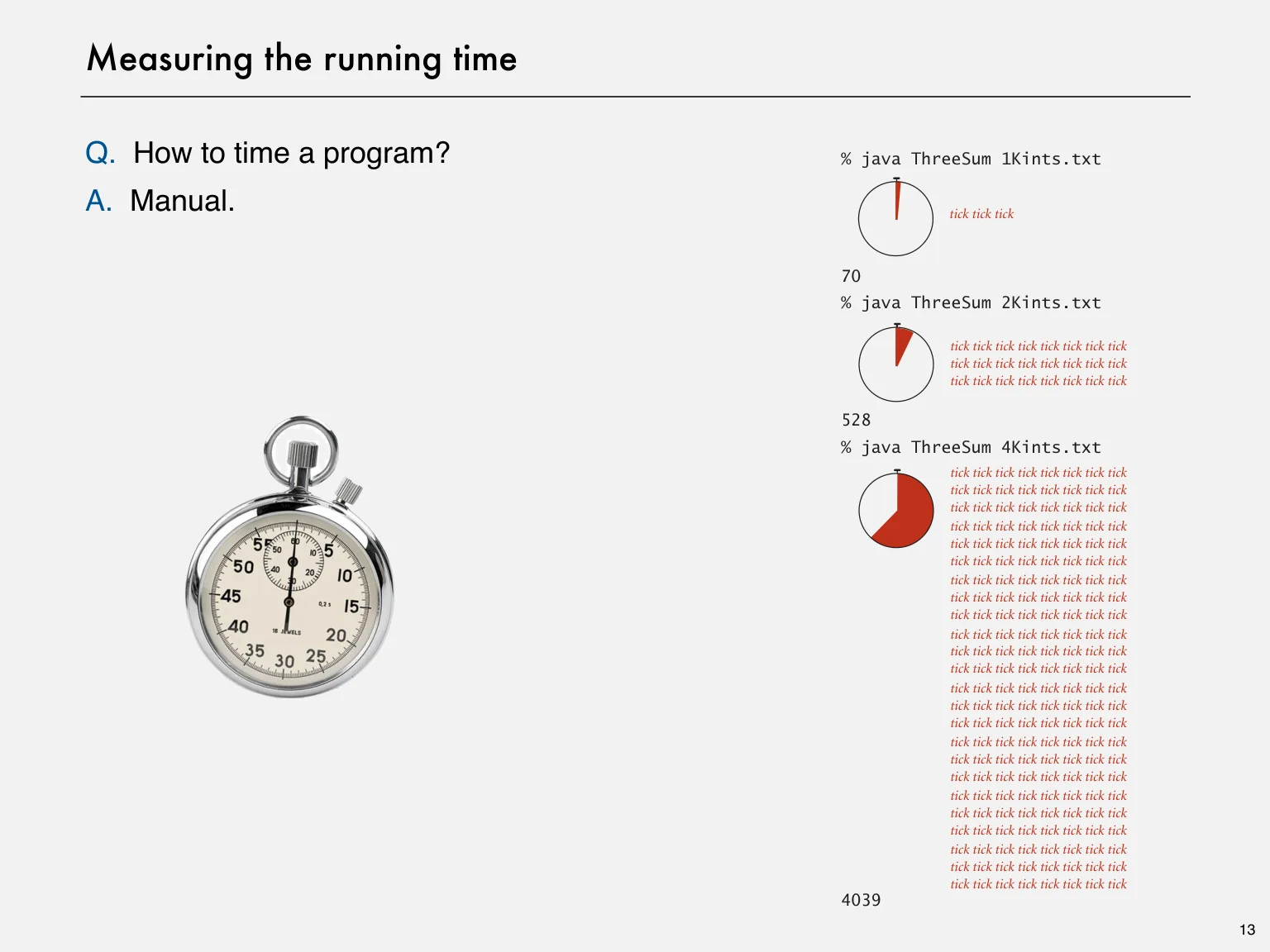
Page 14 · Measuring the running timeOriginal page 14 · Open the image for full detail.
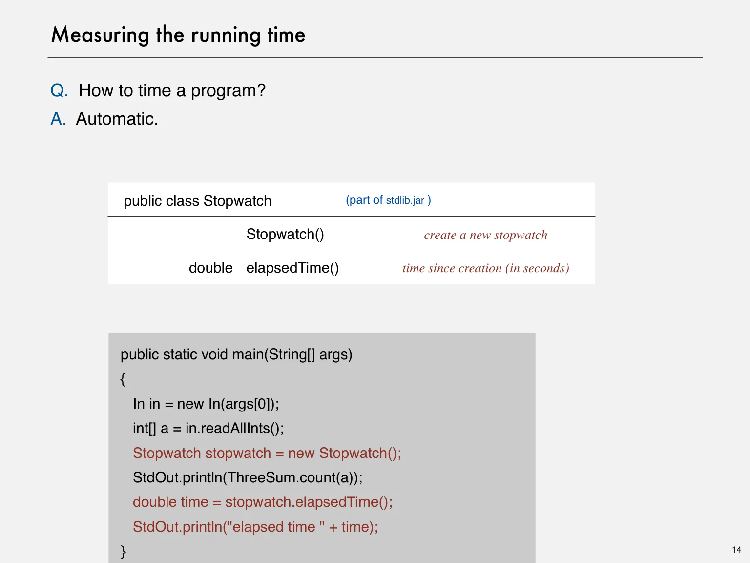
Measuring the running time
Q. How to time a program?
A. Automatic.
public class Stopwatch (part of stdlib.jar )
Stopwatch() create a new stopwatch
double elapsedTime() time since creation (in seconds)
public static void main(String[] args)
{
In in = new In(args[0]);
int[] a = in.readAllInts();
Stopwatch stopwatch = new Stopwatch(); client code
StdOut.println(ThreeSum.count(a));
double time = stopwatch.elapsedTime();
StdOut.println("elapsed time " + time);
} 14
Page 15 · Empirical analysisOriginal page 15 · Open the image for full detail.
Empirical analysis
Run the program for various input sizes and measure running time.
15
Page 16 · Empirical analysisOriginal page 16 · Open the image for full detail.
Empirical analysis
Run the program for various input sizes and measure running time.
N time (seconds) †
250 0
500 0
1,000 0.1
2,000 0.8
4,000 6.4
8,000 51.1
16,000 ?
16
Page 17 · Data analysisOriginal page 17 · Open the image for full detail.
Data analysis
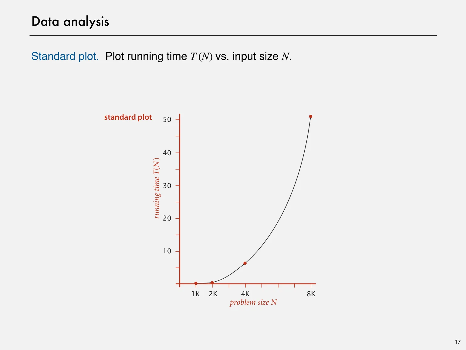
Standard plot. Plot running time T (N) vs. input size N.
standard plot 50
40
T(N)
30 time
running 20
10
1K 2K 4K 8K
problem size N
17
Page 18 · analysisOriginal page 18 · Open the image for full detail.
analysis
Log-log plot. Plot running time T (N) vs. input size N using log-log scale.
log-log plot 51.2 straight line
of slope 3
25.6
12.8 lg(T (N)) = b lg N + c
6.4 b = 2.999
c = -33.2103 3.2 lg(T(N)) 1.6
T (N) = a N b, where a = 2 c
.8
.4
3 orders
.2 of magnitude
.1
1K 2K 4K 8K
lgN
power law
slope
Regression. Fit straight line through data points: a N b.
18 2.999 seconds. Hypothesis. The running time is about 1.006 × 10 –10 × N
Page 19 · Prediction and validationOriginal page 19 · Open the image for full detail.
Prediction and validation
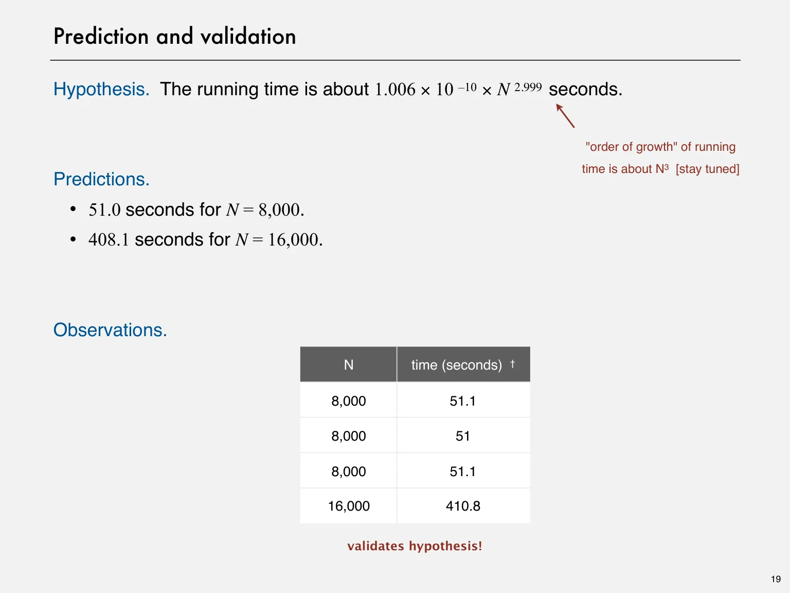
2.999 seconds.Hypothesis. The running time is about 1.006 × 10 –10 × N
"order of growth" of running
time is about N3 [stay tuned]
Predictions.
seconds for N = 8,000.・51.0
seconds for N = 16,000.・408.1
Observations.
N time (seconds) †
8,000 51.1
8,000 51
8,000 51.1
16,000 410.8
validates hypothesis!
19
Page 20 · Doubling hypothesisOriginal page 20 · Open the image for full detail.
Doubling hypothesis
Doubling hypothesis. Quick way to estimate b in a power-law relationship.
Run program, doubling the size of the input.
N time (seconds) † ratio lg ratio
T(2N) a(2N)b
=
T(N) aN b 250 0 –
= 2b
500 0 4.8 2.3
1,000 0.1 6.9 2.8
2,000 0.8 7.7 2.9
4,000 6.4 8 3 lg (6.4 / 0.8) = 3.0
8,000 51.1 8 3
seems to converge to a constant b ≈ 3
Hypothesis. Running time is about a N b with b = lg ratio.
Caveat. Cannot identify logarithmic factors with doubling hypothesis.
20
Page 21 · Doubling hypothesisOriginal page 21 · Open the image for full detail.
Doubling hypothesis
Doubling hypothesis. Quick way to estimate b in a power-law relationship.
Q. How to estimate a (assuming we know b) ?
A. Run the program (for a sufficient large value of N) and solve for a.
N time (seconds) †
8,000 51.1
51.1 = a × 80003
8,000 51
⇒ a = 0.998 × 10 –10
8,000 51.1
3 seconds.Hypothesis. Running time is about 0.998 × 10 –10 × N
almost identical hypothesis
to one obtained via linear regression
21
Page 22 · Experimental algorithmicsOriginal page 22 · Open the image for full detail.
Experimental algorithmics
System independent effects.
・Algorithm. determines exponent
data. in power law・Input
determines constant in
System dependent effects.
power law
CPU, memory, cache, …・Hardware:
compiler, interpreter, garbage collector, …・Software:
operating system, network, other apps, …・System:
Bad news. Difficult to get precise measurements.
Good news. Much easier and cheaper than other sciences.
e.g., can run huge number of experiments
22
Page 23 · 1.4 ANALYSIS OFOriginal page 23 · Open the image for full detail.
1.4 ANALYSIS OF
‣ introduction
‣ observations
‣ mathematical modelsAlgorithms
‣ order-of-growth classifications
‣ theory of algorithms
ROBERT SEDGEWICK | KEVIN WAYNE
http://algs4.cs.princeton.edu ‣ memory
Page 24 · Mathematical models for running timeOriginal page 24 · Open the image for full detail.
Mathematical models for running time
Total running time: sum of cost × frequency for all operations.
to analyze program to determine set of operations.・Need
depends on machine, compiler.・Cost
depends on algorithm, input data.・Frequency
Donald Knuth
1974 Turing Award
In principle, accurate mathematical models are available.
24
Page 25 · Cost of basic operationsOriginal page 25 · Open the image for full detail.
Cost of basic operations
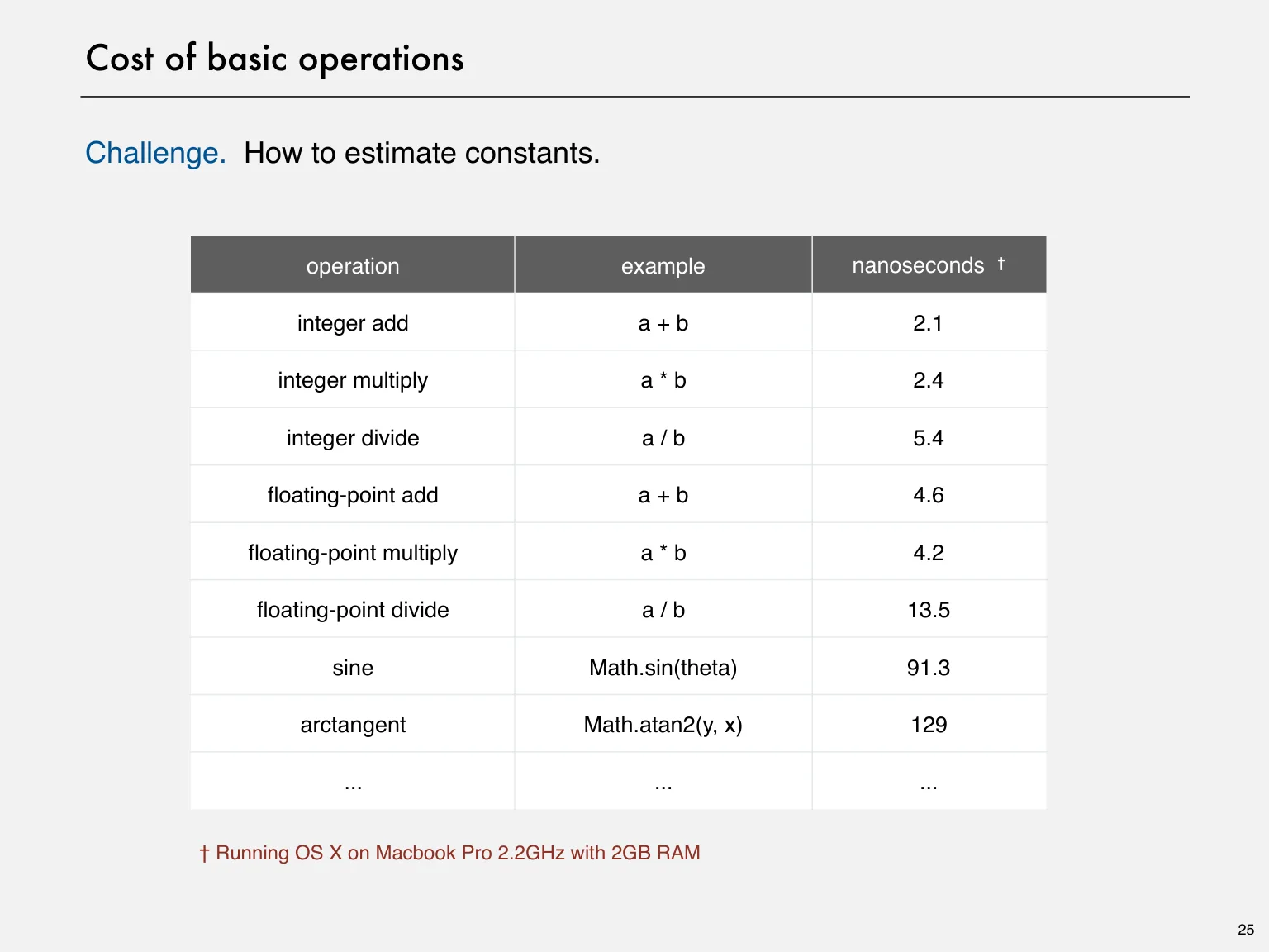
Challenge. How to estimate constants.
operation example nanoseconds †
integer add a + b 2.1
integer multiply a * b 2.4
integer divide a / b 5.4
floating-point add a + b 4.6
floating-point multiply a * b 4.2
floating-point divide a / b 13.5
sine Math.sin(theta) 91.3
arctangent Math.atan2(y, x) 129
... ... ...
† Running OS X on Macbook Pro 2.2GHz with 2GB RAM
25
Page 26 · Cost of basic operationsOriginal page 26 · Open the image for full detail.
Cost of basic operations
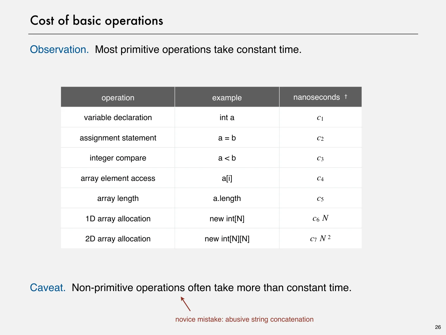
Observation. Most primitive operations take constant time.
operation example nanoseconds †
variable declaration int a c1
assignment statement a = b c2
integer compare a < b c3
array element access a[i] c4
array length a.length c5
1D array allocation new int[N] c6 N
2D array allocation new int[N][N] c7 N 2
Caveat. Non-primitive operations often take more than constant time.
novice mistake: abusive string concatenation
26
Page 27 · Example: 1-SUMOriginal page 27 · Open the image for full detail.
Example: 1-SUM
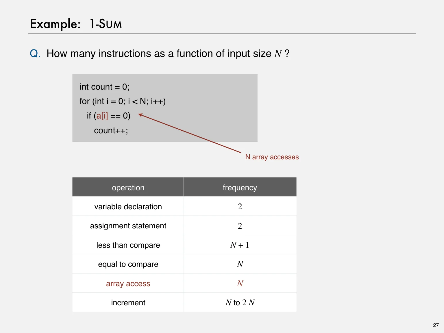
Q. How many instructions as a function of input size N ?
int count = 0;
for (int i = 0; i < N; i++)
if (a[i] == 0)
count++;
N array accesses
operation frequency
variable declaration 2
assignment statement 2
less than compare N + 1
equal to compare N
array access N
increment N to 2 N
27
Page 28 · Example: Frequency Count - SUM IN A ARRAYOriginal page 28 · Open the image for full detail.
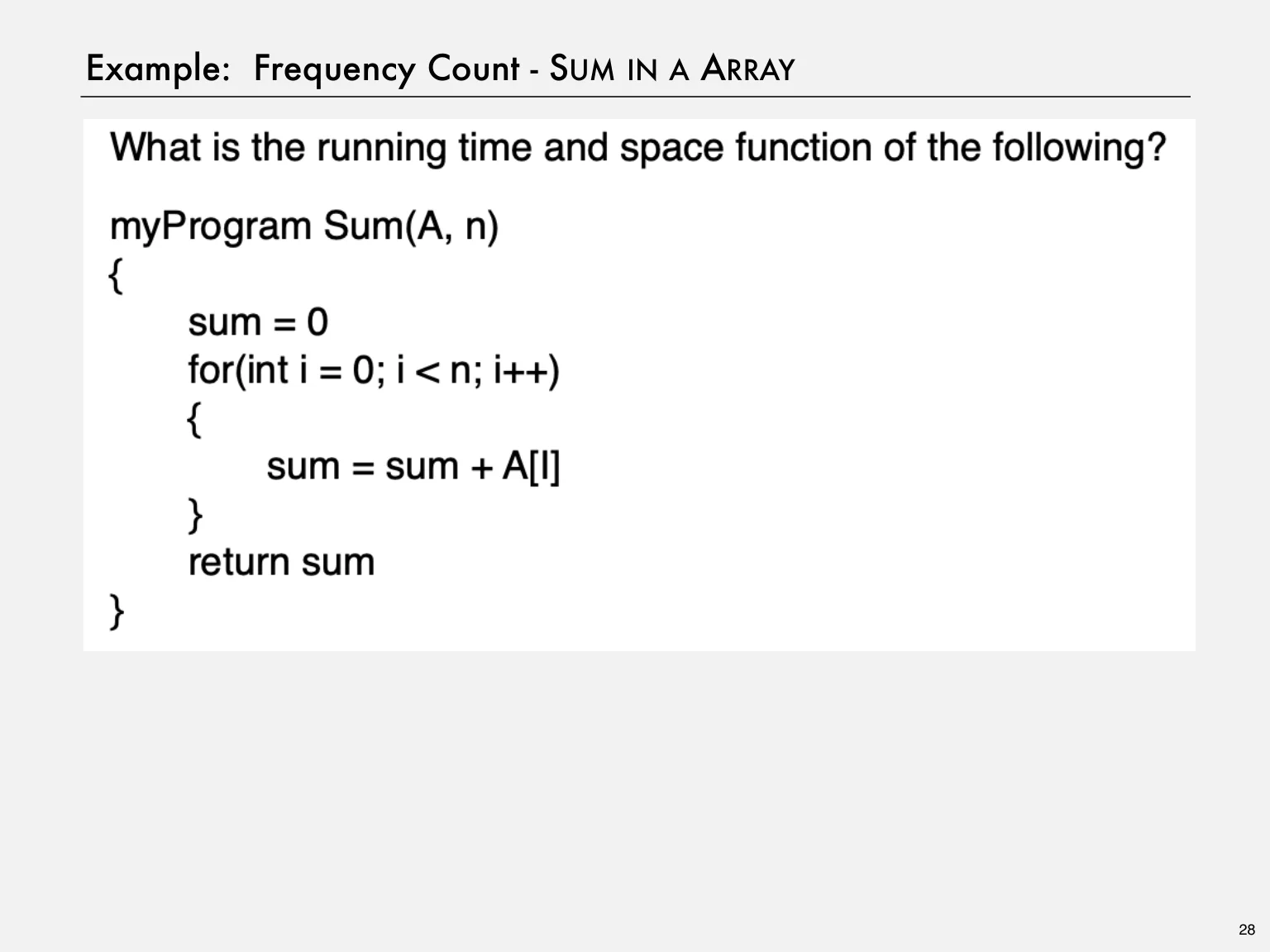
Example: Frequency Count - SUM IN A ARRAY
28
Page 29 · Example: Frequency Count - SUM IN A 2D ARRAYOriginal page 29 · Open the image for full detail.
Example: Frequency Count - SUM IN A 2D ARRAY
29
Page 30 · Example: Frequency Count - Multiplication IN A 2D ARRAYOriginal page 30 · Open the image for full detail.
Example: Frequency Count - Multiplication IN A 2D ARRAY
30
Page 31 · Example: 2-SUMOriginal page 31 · Open the image for full detail.
Example: 2-SUM
Q. How many instructions as a function of input size N ?
int count = 0;
for (int i = 0; i < N; i++)
for (int j = i+1; j < N; j++)
if (a[i] + a[j] == 0)
count++;
1
0 + 1 + 2 + . . . + (N −1) = 2 N (N −1)
Pf. [ n even]
=
2 !N ⇥
1 2
0 + 1 + 2 + . . . + (N −1) = 2N −12N
half of square half of
31
Page 32 · String theory infinite sumOriginal page 32 · Open the image for full detail.
String theory infinite sum
1 + 2 + 3 + 4 + . . . = −112
http://www.nytimes.com/2014/02/04/science/in-the-end-it-all-adds-up-to.html
32
Page 33 · Example: 2-SUMOriginal page 33 · Open the image for full detail.
Example: 2-SUM
Q. How many instructions as a function of input size N ?
int count = 0;
for (int i = 0; i < N; i++)
for (int j = i+1; j < N; j++)
if (a[i] + a[j] == 0)
count++;
1
0 + 1 + 2 + . . . + (N −1) = 2 N (N −1)
=
2 operation frequency !N ⇥
variable declaration N + 2
assignment statement N + 2
less than compare ½ (N + 1) (N + 2)
equal to compare ½ N (N − 1)
tedious to count exactly
array access N (N − 1)
increment ½ N (N − 1) to N (N − 1)
33
Page 34 · Simplifying the calculationsOriginal page 34 · Open the image for full detail.
Simplifying the calculations
“ It is convenient to have a measure of the amount of work involved
in a computing process, even though it be a very crude one. We may
count up the number of times that various elementary operations are
applied in the whole process and then given them various weights.
We might, for instance, count the number of additions, subtractions,
multiplications, divisions, recording of numbers, and extractions
of figures from tables. In the case of computing with matrices most
of the work consists of multiplications and writing down numbers,
and we shall therefore only attempt to count the number of
multiplications and recordings. ” — Alan Turing
ROUNDING-OFF ERRORS IN MATRIX PROCESSES
By A. M. TURING
{National Physical Laboratory, Teddington, Middlesex)
[Received 4 November 1947]
SUMMARY
A number of methods of solving sets of linear equations and inverting matrices
are discussed. The theory of the rounding-off errors involved is investigated for
some of the methods. In all cases examined, including the well-known 'Gauss
elimination process', it is found that the errors are normally quite moderate: no
exponential build-up need occur.
34
Page 35 · Simplification 1: cost modelOriginal page 35 · Open the image for full detail.
Simplification 1: cost model
Cost model. Use some basic operation as a proxy for running time.
int count = 0;
for (int i = 0; i < N; i++)
for (int j = i+1; j < N; j++)
if (a[i] + a[j] == 0)
count++;
1
0 + 1 + 2 + . . . + (N −1) = 2 N (N −1)
=
2 operation frequency !N ⇥
variable declaration N + 2
assignment statement N + 2
less than compare ½ (N + 1) (N + 2)
equal to compare ½ N (N − 1)
array access N (N − 1) cost model = array accesses
(we assume compiler/JVM do not increment ½ N (N − 1) to N (N − 1)
optimize any array accesses away!)
35
Page 36 · Simplification 2: tilde notationOriginal page 36 · Open the image for full detail.
Simplification 2: tilde notation
running time (or memory) as a function of input size N.・Estimate
lower order terms.・Ignore
– when N is large, terms are negligible
– when N is small, we don't care
N 3/6
Ex 1. ⅙ N 3 + 20 N + 16 ~ ⅙ N 3
166,666,667 N 3/6 ! N 2/2 + N /3
Ex 2. ⅙ N 3 + 100 N 4/3 + 56 ~ ⅙ N 3
166,167,000Ex 3. ⅙ N 3 - ½ N 2 + ⅓ N ~ ⅙ N 3
N 1,000
discard lower-order terms Leading-term approximation
(e.g., N = 1000: 166.67 million vs. 166.17 million)
Technical definition. f(N) ~ g(N) means
36
Page 37 · Simplification 2: tilde notationOriginal page 37 · Open the image for full detail.
Simplification 2: tilde notation
running time (or memory) as a function of input size N. ・Estimate
lower order terms. ・Ignore
– when N is large, terms are negligible
– when N is small, we don't care
operation frequency tilde notation
variable declaration N + 2 ~ N
assignment statement N + 2 ~ N
less than compare ½ (N + 1) (N + 2) ~ ½ N 2
equal to compare ½ N (N − 1) ~ ½ N 2
array access N (N − 1) ~ N 2
increment ½ N (N − 1) to N (N − 1) ~ ½ N 2 to ~ N 2
37
Page 38 · Example: 2-SUMOriginal page 38 · Open the image for full detail.
Example: 2-SUM
Q. Approximately how many array accesses as a function of input size N ?
int count = 0;
for (int i = 0; i < N; i++)
for (int j = i+1; j < N; j++)
"inner loop"
if (a[i] + a[j] == 0)
count++;
1
0 + 1 + 2 + . . . + (N −1) = 2 N (N −1)
=
2 !N ⇥
A. ~ N 2 array accesses.
Bottom line. Use cost model and tilde notation to simplify counts.
38
Page 39 · Example: 3-SUMOriginal page 39 · Open the image for full detail.
Example: 3-SUM
Q. Approximately how many array accesses as a function of input size N ?
int count = 0;
for (int i = 0; i < N; i++)
for (int j = i+1; j < N; j++)
for (int k = j+1; k < N; k++) "inner loop"
if (a[i] + a[j] + a[k] == 0)
count++;
N(N = −1)(N −2)
3 3! !N ⇥
A. ~ ½ N 3 array accesses. 1 3
⇥ 6N
Bottom line. Use cost model and tilde notation to simplify counts.
39
Page 40 · Diversion: estimating a discrete sumOriginal page 40 · Open the image for full detail.
Diversion: estimating a discrete sum
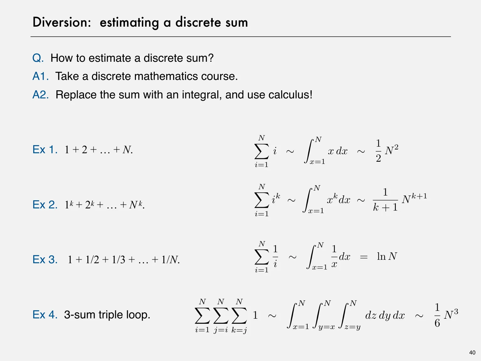
Q. How to estimate a discrete sum?
A1. Take a discrete mathematics course.
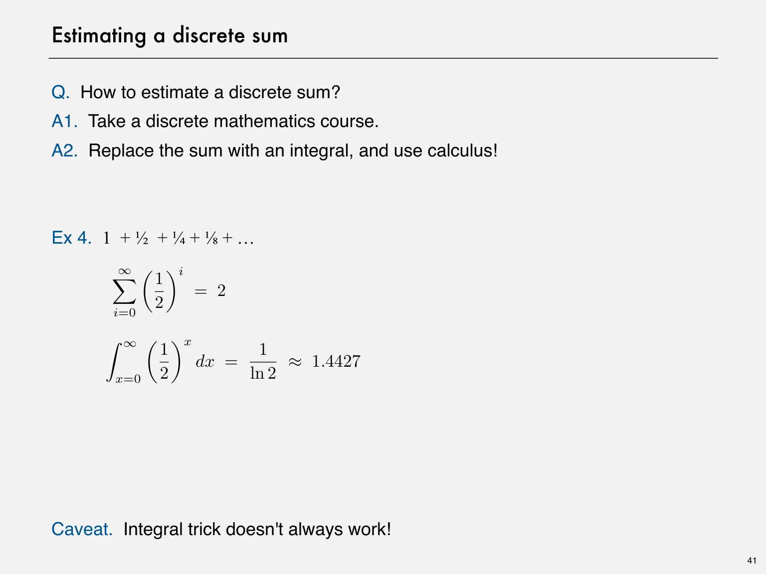
A2. Replace the sum with an integral, and use calculus!
N
1
Ex 1. 1 + 2 + … + N. i x dx N 2
2 ∼ x=1 ∼ i=1 ⇥N !
N N
1
ik xkdx N k+1Ex 2. 1k + 2k + … + N k. k + 1 ∼ x=1 ∼ i=1 " !
N 1 1
= ln NEx 3. 1 + 1/2 + 1/3 + … + 1/N. i ∼ x=1 xdx i=1 ⇥N !
N N N
1 3Ex 4. 3-sum triple loop. 1 dz dy dx N ∼ ∼ 6 x=1 y=x z=y i=1 j=i k=j ⇥N ⇥N ⇥N ! ! !
40
Page 41 · Estimating a discrete sumOriginal page 41 · Open the image for full detail.
Estimating a discrete sum
Q. How to estimate a discrete sum?
A1. Take a discrete mathematics course.
A2. Replace the sum with an integral, and use calculus!
Ex 4. 1 + ½ + ¼ + ⅛ + …
∞
= 2
2
i=0 "1 #i !
∞ 1
dx = 2 ln 2 ≈1.4427 x=0 ! "1 #x
Caveat. Integral trick doesn't always work!
41
Page 42 · Estimating a discrete sumOriginal page 42 · Open the image for full detail.
Estimating a discrete sum
Q. How to estimate a discrete sum?
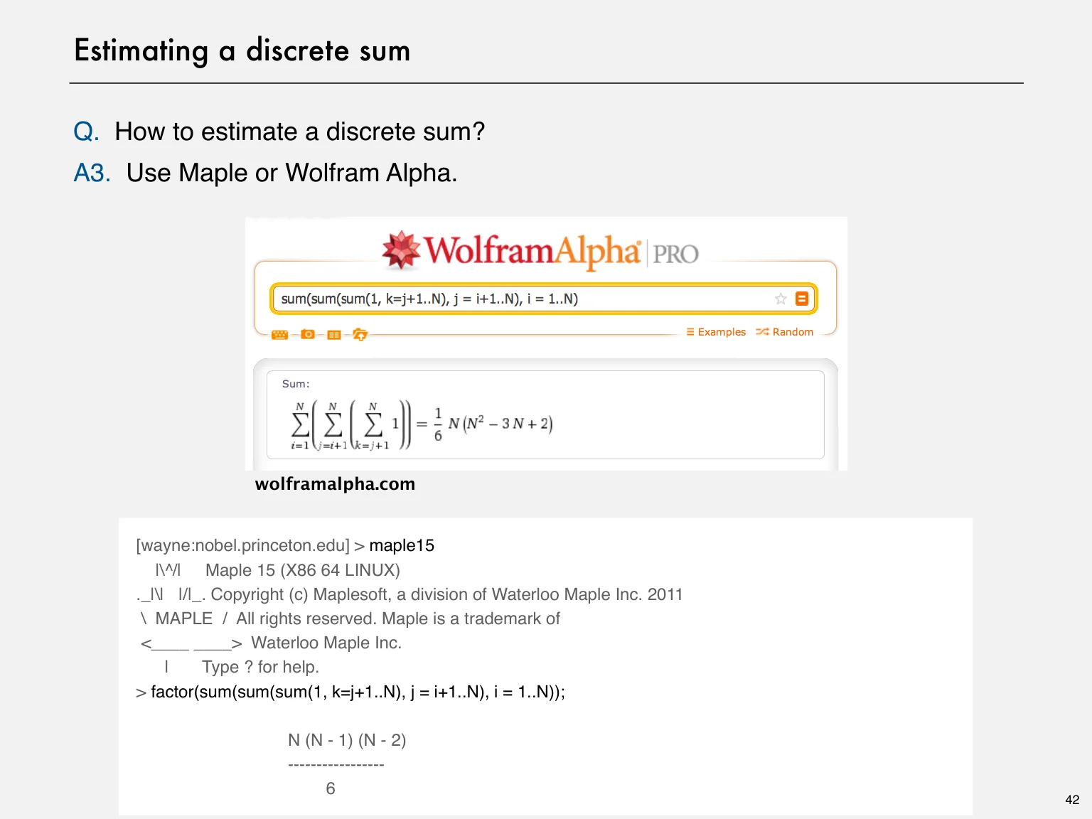
A3. Use Maple or Wolfram Alpha.
wolframalpha.com
[wayne:nobel.princeton.edu] > maple15
|\^/| Maple 15 (X86 64 LINUX)
._|\| |/|_. Copyright (c) Maplesoft, a division of Waterloo Maple Inc. 2011
\ MAPLE / All rights reserved. Maple is a trademark of
<____ ____> Waterloo Maple Inc.
| Type ? for help.
> factor(sum(sum(sum(1, k=j+1..N), j = i+1..N), i = 1..N));
N (N - 1) (N - 2)
-----------------
6
42
Page 43 · Mathematical models for running timeOriginal page 43 · Open the image for full detail.
Mathematical models for running time
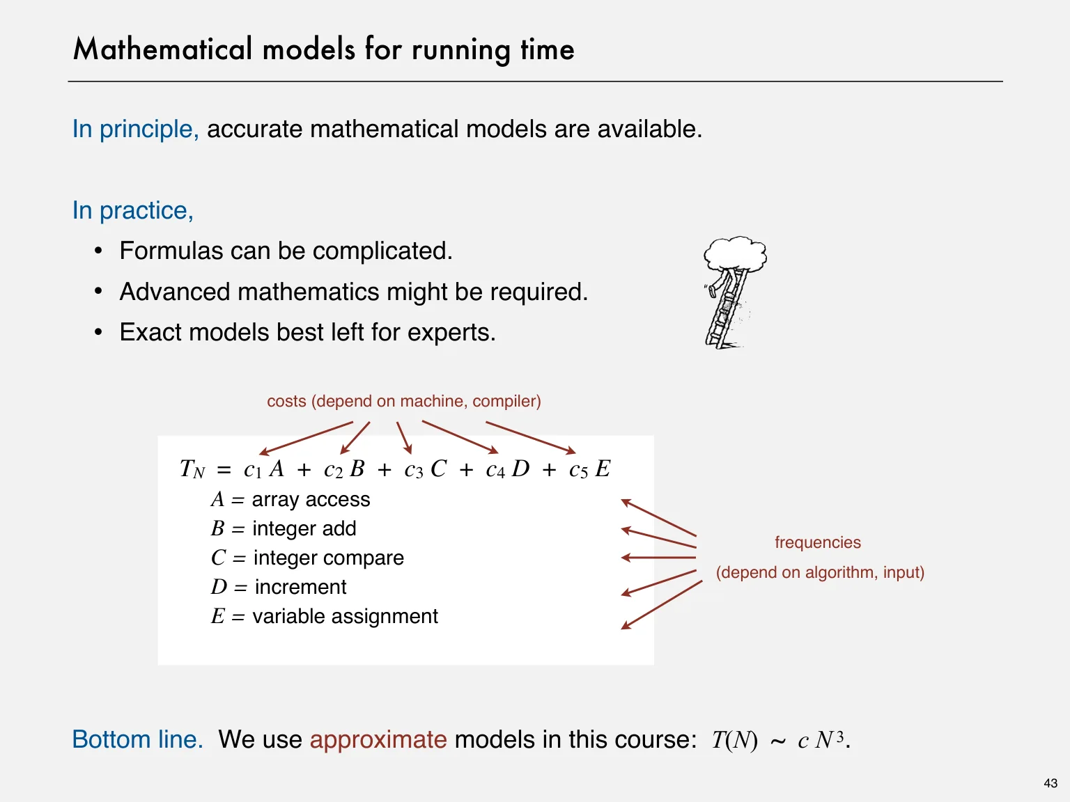
In principle, accurate mathematical models are available.
In practice,
can be complicated.・Formulas
mathematics might be required.・Advanced
models best left for experts.・Exact
costs (depend on machine, compiler)
TN = c1 A + c2 B + c3 C + c4 D + c5 E
A = array access
B = integer add
frequencies
C = integer compare
(depend on algorithm, input)
D = increment
E = variable assignment
Bottom line. We use approximate models in this course: T(N) ~ c N 3.
43
Page 44 · 1.4 ANALYSIS OFOriginal page 44 · Open the image for full detail.
1.4 ANALYSIS OF
‣ introduction
‣ observations
‣ mathematical modelsAlgorithms
‣ order-of-growth classifications
‣ theory of algorithms
ROBERT SEDGEWICK | KEVIN WAYNE
http://algs4.cs.princeton.edu ‣ memory
Page 45 · Common order-of-growth classificationsOriginal page 45 · Open the image for full detail.
Common order-of-growth classifications
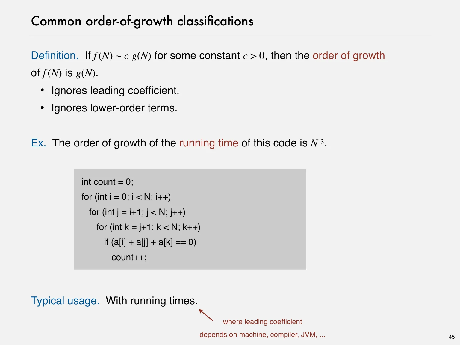
Definition. If f (N) ~ c g(N) for some constant c > 0, then the order of growth
of f (N) is g(N).
leading coefficient.・Ignores
lower-order terms. ・Ignores
Ex. The order of growth of the running time of this code is N 3.
int count = 0;
for (int i = 0; i < N; i++)
for (int j = i+1; j < N; j++)
for (int k = j+1; k < N; k++)
if (a[i] + a[j] + a[k] == 0)
count++;
Typical usage. With running times.
where leading coefficient
depends on machine, compiler, JVM, ... 45
Page 46 · Common order-of-growth classificationsOriginal page 46 · Open the image for full detail.
Common order-of-growth classifications
Good news. The set of functions
1, log N, N, N log N, N 2, N 3, and 2N
suffices to describe the order of growth of most common algorithms.
log-log plot
512T
cubic linear quadratic linearithmic exponential
64T
time
8T
4T
2T
logarithmic
T constant
1K 2K 4K 8K 512K size
Typical orders of growth
46
Page 47 · Common order-of-growth classificationsOriginal page 47 · Open the image for full detail.
Common order-of-growth classifications
order of
name typical code framework description example T(2N) / T(N)
growth
add two
1 constant a = b + c; statement 1
numbers
while (N > 1)
log N logarithmic divide in half binary search ~ 1
{ N = N / 2; ... }
for (int i = 0; i < N; i++) find the
N linear loop 2
{ ... } maximum
divide
N log N linearithmic [see mergesort lecture] mergesort ~ 2
and conquer
for (int i = 0; i < N; i++)
N 2 quadratic for (int j = 0; j < N; j++) double loop check all pairs 4
{ ... }
for (int i = 0; i < N; i++)
for (int j = 0; j < N; j++) check all
N 3 cubic triple loop 8
for (int k = 0; k < N; k++) triples
{ ... }
exhaustive check all
2N exponential [see combinatorial search lecture] T(N)
search subsets
47
Page 48 · Example 1: Common order-of-growth classificationsOriginal page 48 · Open the image for full detail.
Example 1: Common order-of-growth classifications
order of
name typical code framework description example T(2N) / T(N)
growth
add two
1 constant a = b + c; statement 1
numbers
while (N > 1)
log N logarithmic divide in half binary search ~ 1
{ N = N / 2; ... }
for (int i = 0; i < N; i++) find the
N linear loop 2
{ ... } maximum
divide
N log N linearithmic [see mergesort lecture] mergesort ~ 2
and conquer
for (int i = 0; i < N; i++)
N 2 quadratic for (int j = 0; j < N; j++) double loop check all pairs 4
{ ... }
for (int i = 0; i < N; i++)
for (int j = 0; j < N; j++) check all
N 3 cubic triple loop 8
for (int k = 0; k < N; k++) triples
{ ... }
exhaustive check all
2N exponential [see combinatorial search lecture] T(N)
search subsets
48
Page 49 · Example 1: Common order-of-growth classificationsOriginal page 49 · Open the image for full detail.
Example 1: Common order-of-growth classifications
Time: f(n) = 2n + 3
Space: f(n) = n + 3
49
Page 50 · Example 2: Common order-of-growth classificationsOriginal page 50 · Open the image for full detail.
Example 2: Common order-of-growth classifications
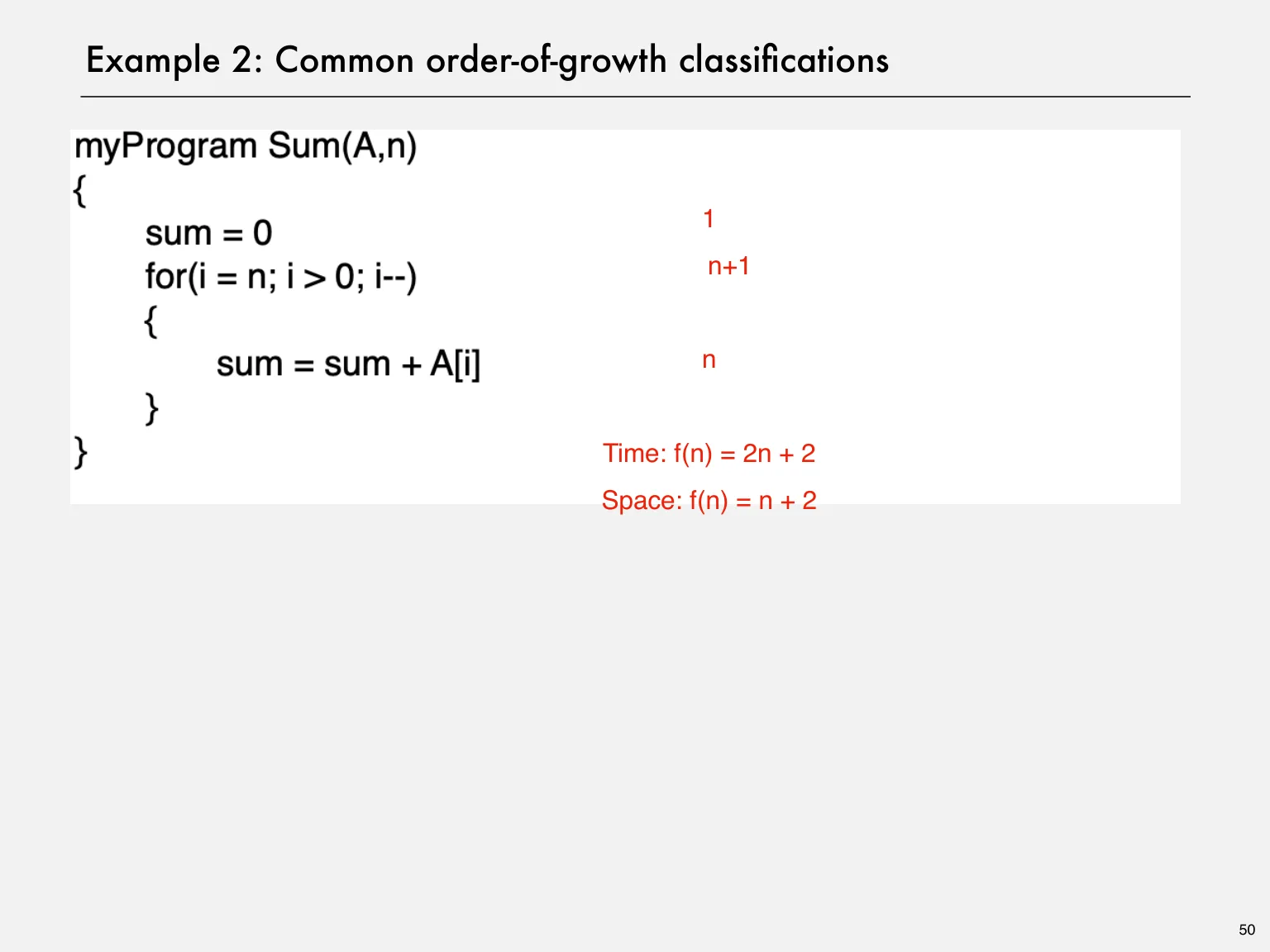
1
n+1
n
Time: f(n) = 2n + 2
Space: f(n) = n + 2
50
Page 51 · Example 3: Common order-of-growth classificationsOriginal page 51 · Open the image for full detail.
Example 3: Common order-of-growth classifications
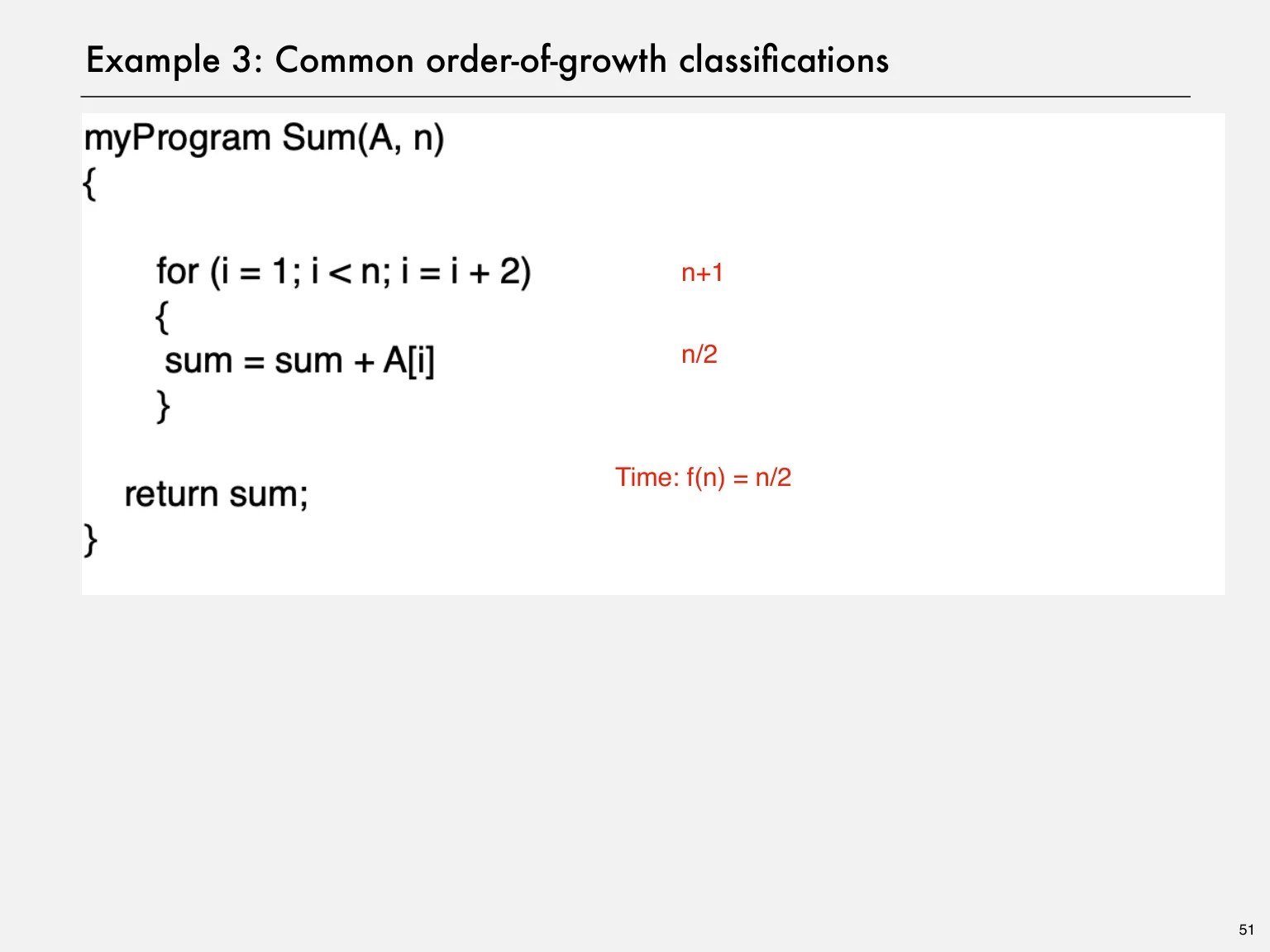
n+1
n/2
Time: f(n) = n/2
51
Page 52 · Example 4: Common order-of-growth classificationsOriginal page 52 · Open the image for full detail.
Example 4: Common order-of-growth classifications
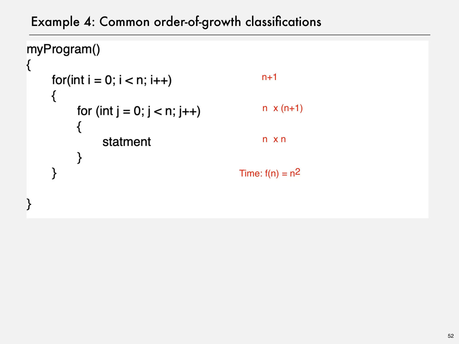
n+1
n x (n+1)
n x n
Time: f(n) = n2
52
Page 53 · Example 5: Common order-of-growth classificationsOriginal page 53 · Open the image for full detail.
Example 5: Common order-of-growth classifications
i j No. Of times
0 0 0
1 0,1 1
2 0,1,2 2
3 0,1,2,3 3
f(n) = 1+2+3+…..+n = n(n+1)/2
53
Page 54 · Example 6: Common order-of-growth classificationsOriginal page 54 · Open the image for full detail.
Example 6: Common order-of-growth classifications
i p
1 0+1
2 1+2
3 1+2+3
4 1+2+3+4
- -
- -
k 1+2+3+4+…k
At p > n loop will break
k(k+1)/2 > n
k2 > n
k > (n)1/2
54
Page 55 · Example 7: Common order-of-growth classificationsOriginal page 55 · Open the image for full detail.
Example 7: Common order-of-growth classifications
55
Page 56 · Example 8: Common order-of-growth classificationsOriginal page 56 · Open the image for full detail.
Example 8: Common order-of-growth classifications
56
Page 57 · Example 9: Common order-of-growth classificationsOriginal page 57 · Open the image for full detail.
Example 9: Common order-of-growth classifications
57
Page 58 · Example 10: Common order-of-growth classificationsOriginal page 58 · Open the image for full detail.
Example 10: Common order-of-growth classifications
58
Page 59 · Example 12: Common order-of-growth classificationsOriginal page 59 · Open the image for full detail.
Example 12: Common order-of-growth classifications
59
Page 60 · Example 13: Common order-of-growth classificationsOriginal page 60 · Open the image for full detail.
Example 13: Common order-of-growth classifications
60
Page 61 · Example 14: Common order-of-growth classificationsOriginal page 61 · Open the image for full detail.
Example 14: Common order-of-growth classifications
61
Page 62 · Example 15: Common order-of-growth classificationsOriginal page 62 · Open the image for full detail.
Example 15: Common order-of-growth classifications
62
Page 63 · Example 16: Common order-of-growth classificationsOriginal page 63 · Open the image for full detail.
Example 16: Common order-of-growth classifications
63
Page 64 · Example 17: Common order-of-growth classificationsOriginal page 64 · Open the image for full detail.
Example 17: Common order-of-growth classifications
64
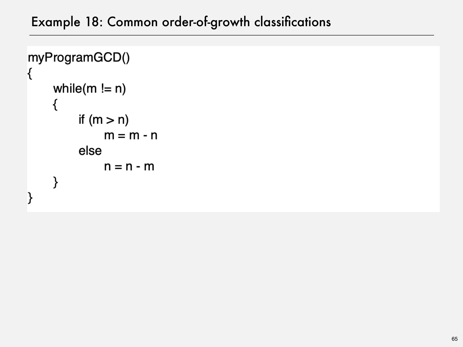
Page 65 · Example 18: Common order-of-growth classificationsOriginal page 65 · Open the image for full detail.
Example 18: Common order-of-growth classifications
65
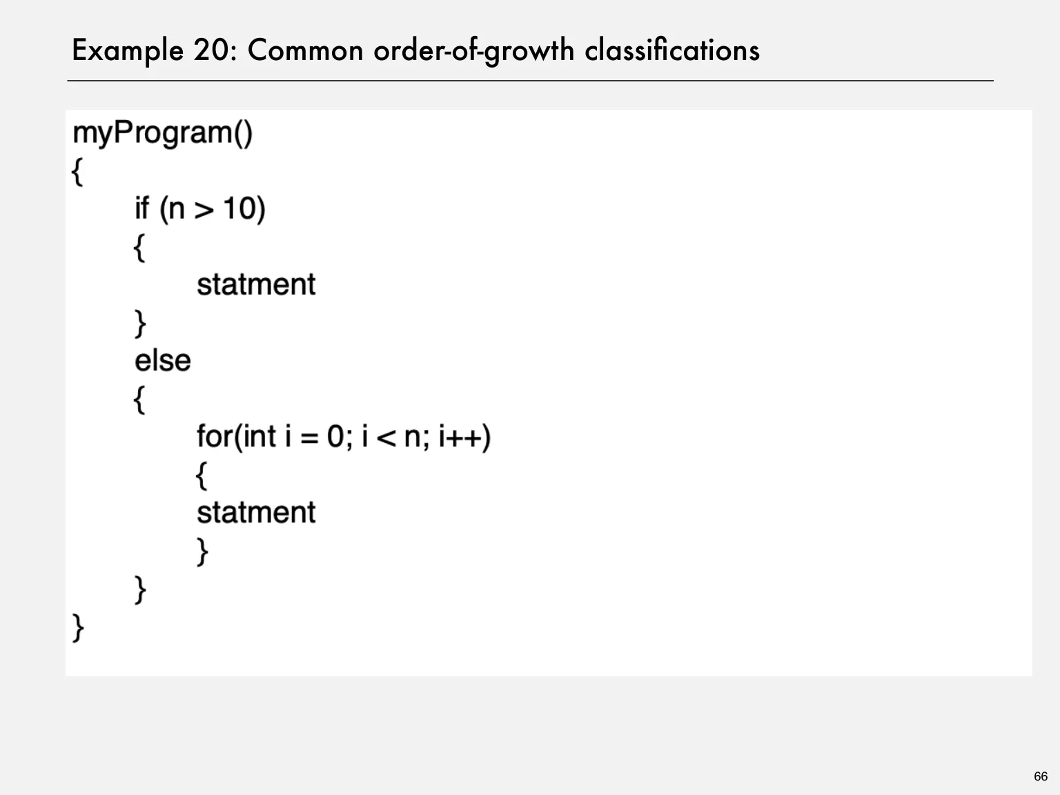
Page 66 · Example 20: Common order-of-growth classificationsOriginal page 66 · Open the image for full detail.
Example 20: Common order-of-growth classifications
66
Page 67 · Example 21: Common order-of-growth classifications 2-SUMOriginal page 67 · Open the image for full detail.
Example 21: Common order-of-growth classifications 2-SUM
int count = 0;
for (int i = 0; i < N; i++)
for (int j = i+1; j < N; j++)
if (a[i] + a[j] == 0)
count++;
67
Page 68 · Binary search demoOriginal page 68 · Open the image for full detail.
Binary search demo
Goal. Given a sorted array and a key, find index of the key in the array?
Binary search. Compare key against middle entry.
small, go left. ・Too
big, go right. ・Too
found. ・Equal,
successful search for 33
6 13 14 25 33 43 51 53 64 72 84 93 95 96 97
0 1 2 3 4 5 6 7 8 9 10 11 12 13 14
lo hi
68
Page 69 · Binary search: Java implementation Trivial to implement?Original page 69 · Open the image for full detail.
Binary search: Java implementation Trivial to implement?
binary search published in 1946. ・First
bug-free one in 1962. ・First
in Java's Arrays.binarySearch() discovered in 2006. ・Bug
public static int binarySearch(int[] a, int key)
{
int lo = 0, hi = a.length-1;
while (lo <= hi)
{
int mid = lo + (hi - lo) / 2;
one "3-way compare" if (key < a[mid]) hi = mid - 1;
else if (key > a[mid]) lo = mid + 1;
else return mid;
}
return -1;
}
Invariant. If key appears in the array a[], then a[lo] ≤ key ≤ a[hi].
69
Page 70 · Binary search: mathematical analysisOriginal page 70 · Open the image for full detail.
Binary search: mathematical analysis
Proposition. Binary search uses at most 1 + lg N key compares to search in a
sorted array of size N.
Def. T (N) = # key compares to binary search a sorted subarray of size ≤ N.
Binary search recurrence. T (N) ≤ T (N / 2) + 1 for N > 1, with T (1) = 1.
left or right half possible to implement with one
(floored division) 2-way compare (instead of 3-way)
Pf sketch. [assume N is a power of 2]
T (N) ≤ T (N / 2) + 1 [ given ]
≤ T (N / 4) + 1 + 1 [ apply recurrence to first term ]
≤ T (N / 8) + 1 + 1 + 1 [ apply recurrence to first term ]
⋮
≤ T (N / N) + 1 + 1 + … + 1 [ stop applying, T(1) = 1 ]
= 1 + lg N
70
Page 71 · An N2 log N algorithm for 3-SUMOriginal page 71 · Open the image for full detail.
An N2 log N algorithm for 3-SUM
inputAlgorithm.
30 -40 -20 -10 40 0 10 5
1: Sort the N (distinct) numbers.・Step
2: For each pair of numbers a[i] sort・Step
-40 -20 -10 0 5 10 30 40 and a[j], binary search for -(a[i] + a[j]).
binary search
(-40, -20) 60
Analysis. Order of growth is N 2 log N.
(-40, -10) 50
1: N 2 with insertion sort.・Step (-40, 0) 40
2: N 2 log N with binary search.・Step (-40, 5) 35
(-40, 10) 30
⋮ ⋮
Remark. Can achieve N 2 by modifying (-20, -10) 30
binary search step. ⋮ ⋮ only count if
a[i] < a[j] < a[k]
(-10, 0) 10
to avoid
⋮ ⋮ double counting
( 10, 30) -40
71
( 10, 40) -50
Page 72 · Comparing programsOriginal page 72 · Open the image for full detail.
Comparing programs
Hypothesis. The sorting-based N 2 log N algorithm for 3-SUM is significantly faster in
practice than the brute-force N 3 algorithm.
N time (seconds) N time (seconds)
1,000 0.1 1,000 0.14
2,000 0.8 2,000 0.18
4,000 6.4 4,000 0.34
8,000 51.1 8,000 0.96
ThreeSum.java 16,000 3.67
32,000 14.88
64,000 59.16
ThreeSumDeluxe.java
Guiding principle. Typically, better order of growth ⇒ faster in practice.
72
Page 73 · 1.4 ANALYSIS OFOriginal page 73 · Open the image for full detail.
1.4 ANALYSIS OF
‣ introduction
‣ observations
‣ mathematical modelsAlgorithms
‣ order-of-growth classifications
‣ theory of algorithms
ROBERT SEDGEWICK | KEVIN WAYNE
http://algs4.cs.princeton.edu ‣ memory
Page 74 · Types of analysesOriginal page 74 · Open the image for full detail.
Types of analyses
Best case. Lower bound on cost.
by “easiest” input.・Determined
a goal for all inputs.・Provides
Worst case. Upper bound on cost.
by “most difficult” input.・Determined
a guarantee for all inputs.・Provides
this course
Average case. Expected cost for random input.
a model for “random” input.・Need
a way to predict performance.・Provides
Ex 1. Array accesses for brute-force 3-SUM. Ex 2. Compares for binary search.
Best: ~ ½ N 3 Best: ~ 1
Average: ~ ½ N 3 Average: ~ lg N
Worst: ~ ½ N 3 Worst: ~ lg N
74
Page 75 · Theory of algorithmsOriginal page 75 · Open the image for full detail.
Theory of algorithms
Goals.
“difficulty” of a problem.・Establish
“optimal” algorithms.・Develop
Approach.
details in analysis: analyze “to within a constant factor.”・Suppress
variability in input model: focus on the worst case.・Eliminate
Upper bound. Performance guarantee of algorithm for any input.
Lower bound. Proof that no algorithm can do better.
Optimal algorithm. Lower bound = upper bound (to within a constant factor).
75
Page 76 · Commonly-used notations in the theory of algorithmsOriginal page 76 · Open the image for full detail.
Commonly-used notations in the theory of algorithms
notation provides example shorthand for used to
½ N 2
asymptotic 10 N 2 classify
Big Theta Θ(N2)
order of growth 5 N 2 + 22 N log N + 3N algorithms
⋮
10 N 2
100 N develop
Big Oh Θ(N2) and smaller O(N2)
22 N log N + 3 N upper bounds
⋮
½ N 2
N 5 develop
Big Omega Θ(N2) and larger Ω(N2)
N 3 + 22 N log N + 3 N lower bounds
⋮
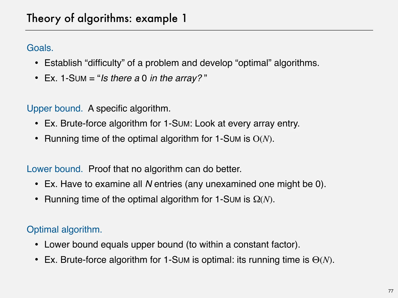
Page 77 · Theory of algorithms: example 1Original page 77 · Open the image for full detail.
Theory of algorithms: example 1
Goals.
“difficulty” of a problem and develop “optimal” algorithms.・Establish
1-SUM = “Is there a 0 in the array? ”・Ex.
Upper bound. A specific algorithm.
Brute-force algorithm for 1-SUM: Look at every array entry.・Ex.
time of the optimal algorithm for 1-SUM is O(N).・Running
Lower bound. Proof that no algorithm can do better.
Have to examine all N entries (any unexamined one might be 0).・Ex.
time of the optimal algorithm for 1-SUM is Ω(N).・Running
Optimal algorithm.
bound equals upper bound (to within a constant factor).・Lower
Brute-force algorithm for 1-SUM is optimal: its running time is Θ(N).・Ex.
77
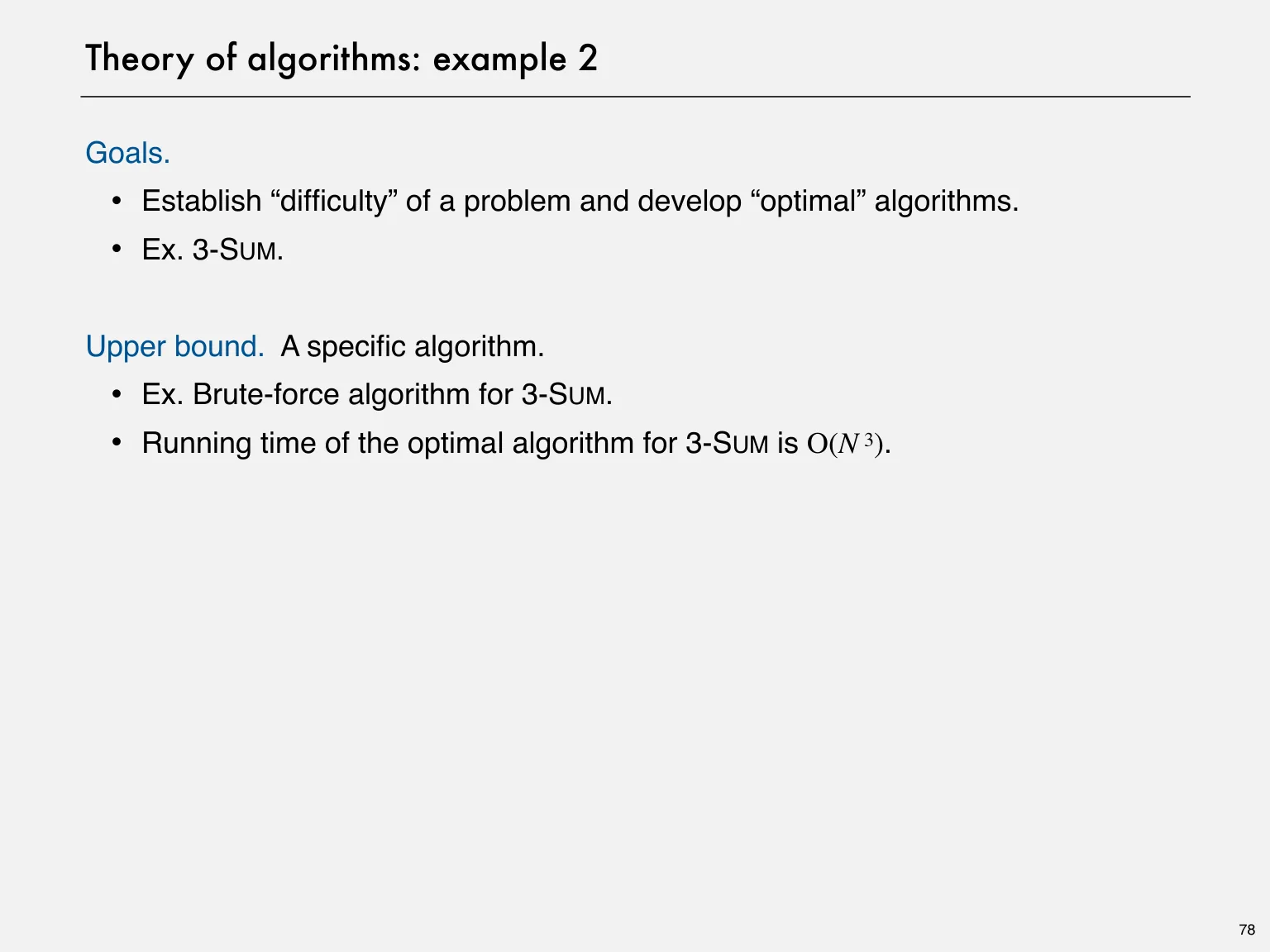
Page 78 · Theory of algorithms: example 2Original page 78 · Open the image for full detail.
Theory of algorithms: example 2
Goals.
“difficulty” of a problem and develop “optimal” algorithms.・Establish
3-SUM.・Ex.
Upper bound. A specific algorithm.
Brute-force algorithm for 3-SUM.・Ex.
time of the optimal algorithm for 3-SUM is O(N 3).・Running
78
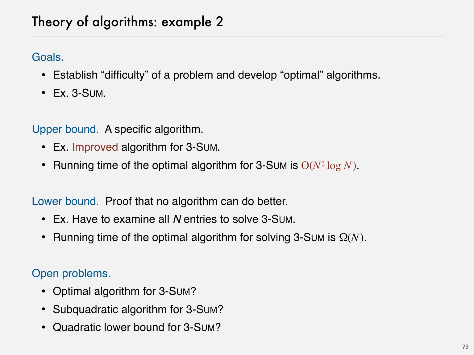
Page 79 · Theory of algorithms: example 2Original page 79 · Open the image for full detail.
Theory of algorithms: example 2
Goals.
“difficulty” of a problem and develop “optimal” algorithms.・Establish
3-SUM.・Ex.
Upper bound. A specific algorithm.
Improved algorithm for 3-SUM.・Ex.
time of the optimal algorithm for 3-SUM is O(N 2 log N ).・Running
Lower bound. Proof that no algorithm can do better.
Have to examine all N entries to solve 3-SUM.・Ex.
time of the optimal algorithm for solving 3-SUM is Ω(N ).・Running
Open problems.
algorithm for 3-SUM?・Optimal
algorithm for 3-SUM?・Subquadratic
lower bound for 3-SUM?・Quadratic
79
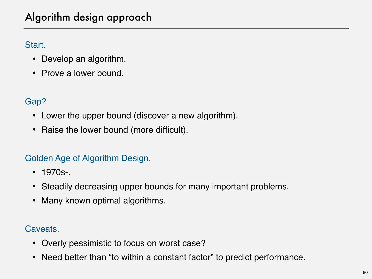
Page 80 · Algorithm design approachOriginal page 80 · Open the image for full detail.
Algorithm design approach
Start.
an algorithm.・Develop
a lower bound.・Prove
Gap?
the upper bound (discover a new algorithm).・Lower
the lower bound (more difficult).・Raise
Golden Age of Algorithm Design.
・1970s‑.
decreasing upper bounds for many important problems.・Steadily
known optimal algorithms.・Many
Caveats.
pessimistic to focus on worst case?・Overly
better than “to within a constant factor” to predict performance.・Need
80
Page 81 · Commonly-used notations in the theory of algorithmsOriginal page 81 · Open the image for full detail.
Commonly-used notations in the theory of algorithms
notation provides example shorthand for used to
10 N 2
provide
2 10 N 2 + 22 N log N Tilde leading term ~ 10 N
approximate model
10 N 2 + 2 N + 37
½ N 2
asymptotic classify
Big Theta Θ(N2) 10 N 2
order of growth algorithms
5 N 2 + 22 N log N + 3N
10 N 2
develop
Big Oh Θ(N2) and smaller O(N2) 100 N
upper bounds
22 N log N + 3 N
½ N 2
develop
5 Big Omega Θ(N2) and larger Ω(N2) N
lower bounds
N 3 + 22 N log N + 3 N
Common mistake. Interpreting big-Oh as an approximate model.
This course. Focus on approximate models: use Tilde-notation
81
Page 82 · 1.4 ANALYSIS OFOriginal page 82 · Open the image for full detail.
1.4 ANALYSIS OF
‣ introduction
‣ observations
‣ mathematical modelsAlgorithms
‣ order-of-growth classifications
‣ theory of algorithms
ROBERT SEDGEWICK | KEVIN WAYNE
http://algs4.cs.princeton.edu ‣ memory
Page 83 · BasicsOriginal page 83 · Open the image for full detail.
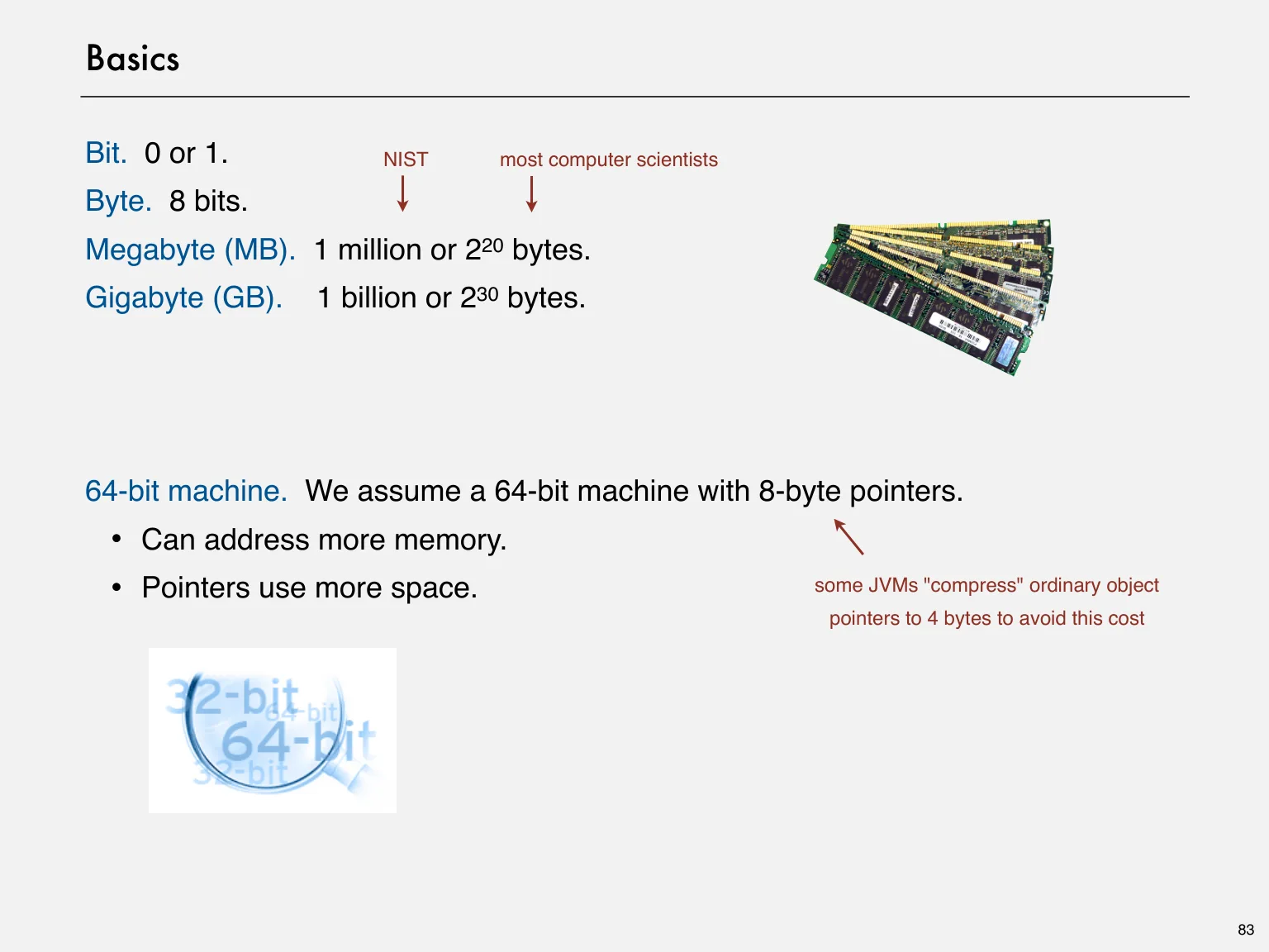
Basics
Bit. 0 or 1. NIST most computer scientists
Byte. 8 bits.
Megabyte (MB). 1 million or 220 bytes.
Gigabyte (GB). 1 billion or 230 bytes.
64-bit machine. We assume a 64-bit machine with 8-byte pointers.
address more memory.・Can
use more space. some JVMs "compress" ordinary object・Pointers
pointers to 4 bytes to avoid this cost
83
Page 84 · Typical memory usage for primitive types and arraysOriginal page 84 · Open the image for full detail.
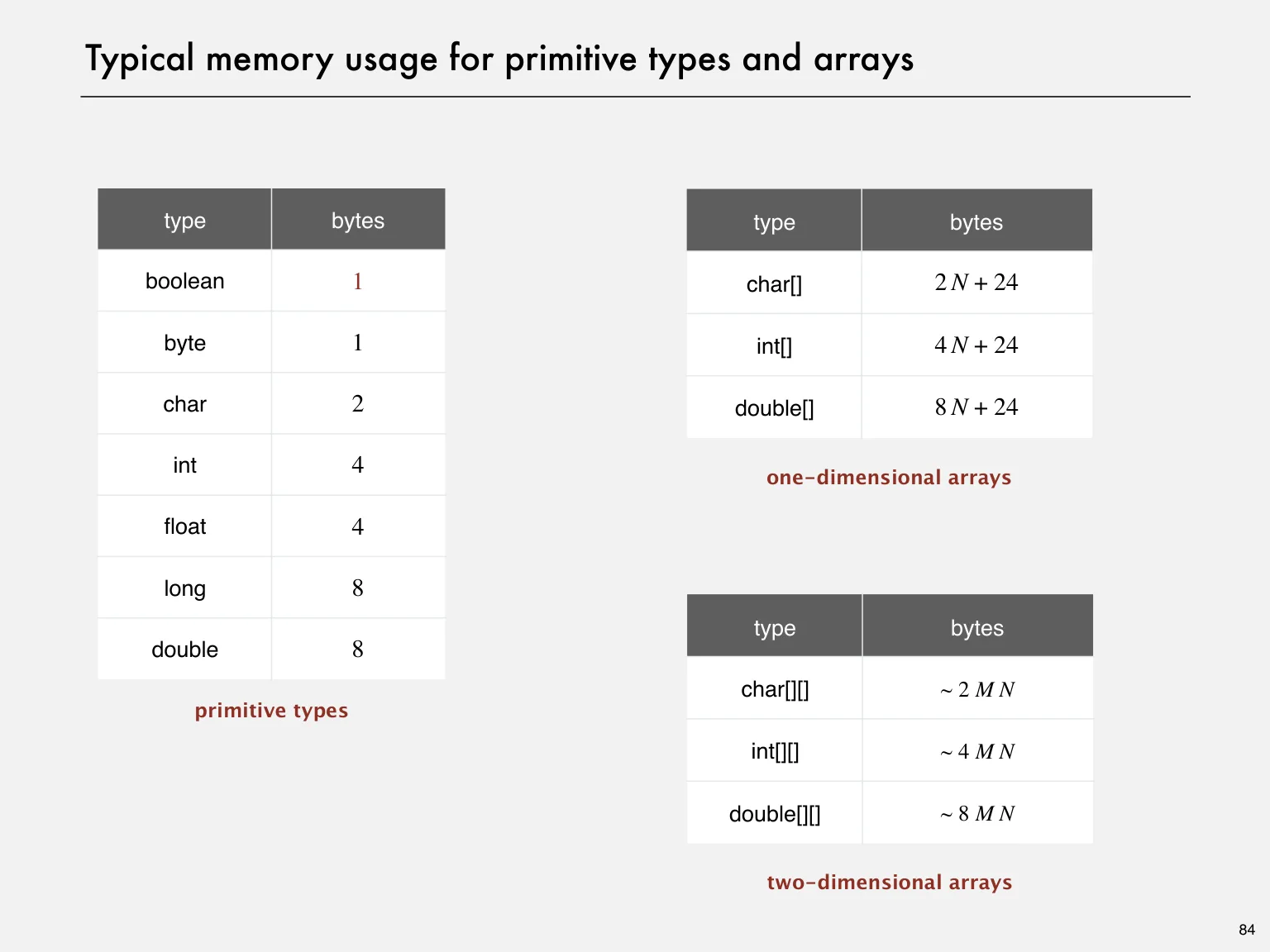
Typical memory usage for primitive types and arrays
type bytes type bytes
boolean 1 char[] 2 N + 24
byte 1 int[] 4 N + 24
char 2 double[] 8 N + 24
int 4 one-dimensional arrays
float 4
long 8
type bytes
double 8
char[][] ~ 2 M N
primitive types
int[][] ~ 4 M N
double[][] ~ 8 M N
two-dimensional arrays
84
Page 85 · Typical memory usage for objects in JavaOriginal page 85 · Open the image for full detail.
Typical memory usage for objects in Java
Object overhead. 16 bytes.
Reference. 8 bytes.
Padding. Each object uses a multiple of 8 bytes.
Ex 1. A Date object uses 32 bytes of memory.
public class Date
{
private int day; object 16 bytes (object overhead)
private int month; overhead
private int year;
...
} day 4 bytes (int)
int month 4 bytes (int)
values year 4 bytes (int)
padding 4 bytes (padding)
32 bytes
85
Page 86 · Typical memory usage summaryOriginal page 86 · Open the image for full detail.
Typical memory usage summary
Total memory usage for a data type value:
type: 4 bytes for int, 8 bytes for double, …・Primitive
reference: 8 bytes.・Object
24 bytes + memory for each array entry.・Array:
16 bytes + memory for each instance variable.・Object:
round up to multiple of 8 bytes.・Padding:
+ 8 extra bytes per inner class object
(for reference to enclosing class)
Shallow memory usage: Don't count referenced objects.
Deep memory usage: If array entry or instance variable is a reference,
count memory (recursively) for referenced object.
86
Page 87 · ExampleOriginal page 87 · Open the image for full detail.
Example
Q. How much memory does WeightedQuickUnionUF use as a function of N ?
Use tilde notation to simplify your answer.
16 bytes
public class WeightedQuickUnionUF
(object overhead)
{
8 + (4N + 24) bytes each
private int[] id;
(reference + int[] array)
private int[] sz; 4 bytes (int)
private int count; 4 bytes (padding)
8N + 88 bytes
public WeightedQuickUnionUF(int N)
{
id = new int[N];
sz = new int[N];
for (int i = 0; i < N; i++) id[i] = i;
for (int i = 0; i < N; i++) sz[i] = 1;
}
A. 8 N + 88 ~ 8 N bytes.
87
Page 88 · Turning the crank: summaryOriginal page 88 · Open the image for full detail.
Turning the crank: summary
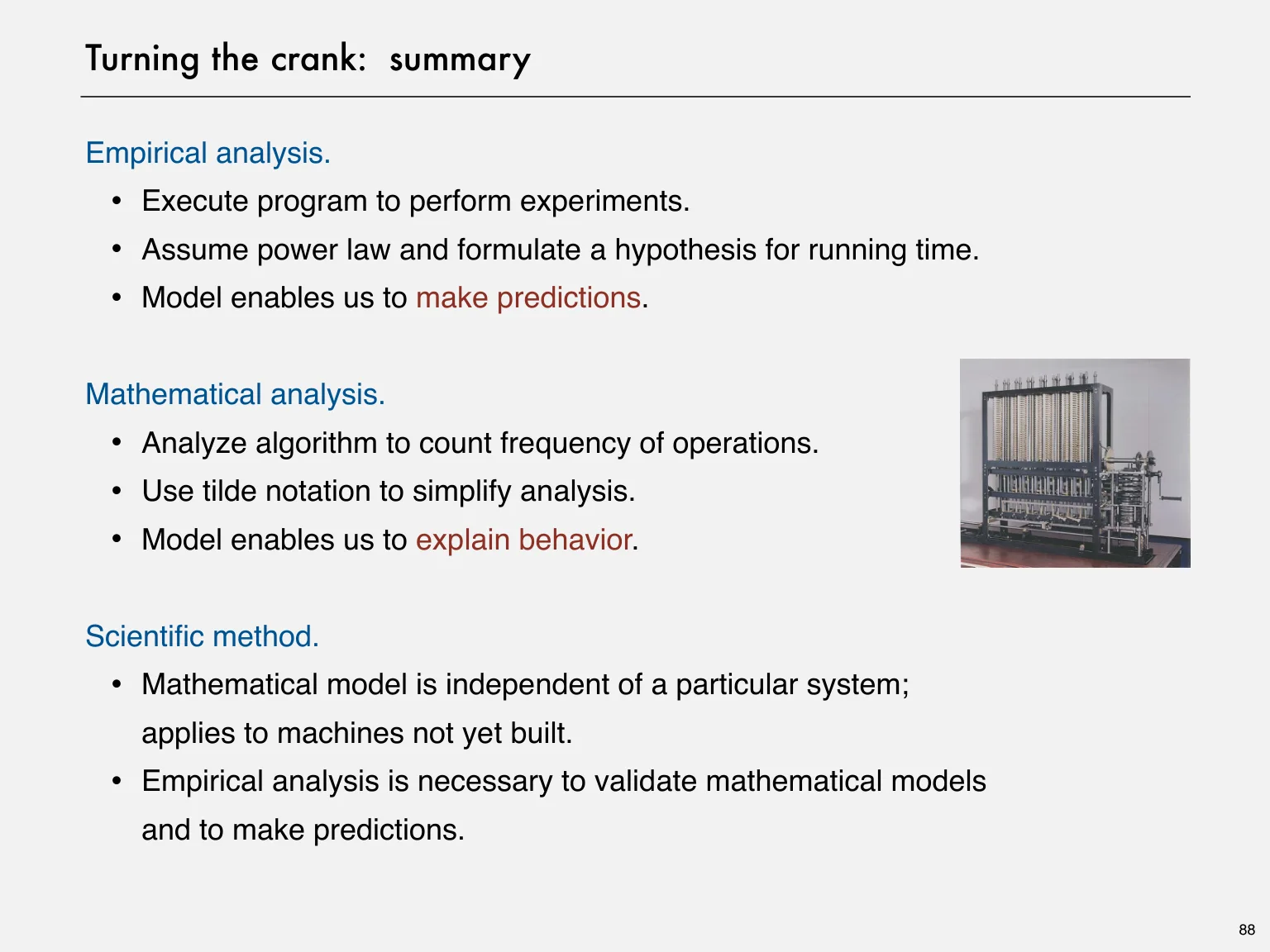
Empirical analysis.
program to perform experiments.・Execute
power law and formulate a hypothesis for running time.・Assume
enables us to make predictions.・Model
Mathematical analysis.
algorithm to count frequency of operations.・Analyze
tilde notation to simplify analysis.・Use
enables us to explain behavior.・Model
Scientific method.
model is independent of a particular system; ・Mathematical
applies to machines not yet built.
analysis is necessary to validate mathematical models ・Empirical
and to make predictions.
88