Course navigation & on this pageLecture 05 · CS-702
Union–find & dynamic connectivity
Improve a connectivity data structure from eager component labels to weighted trees and path compression.
Intermediate~65 min guideSource-based learning
What you’ll understand
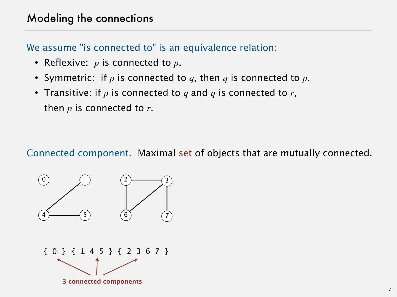
Model connectivity as an equivalence relation.
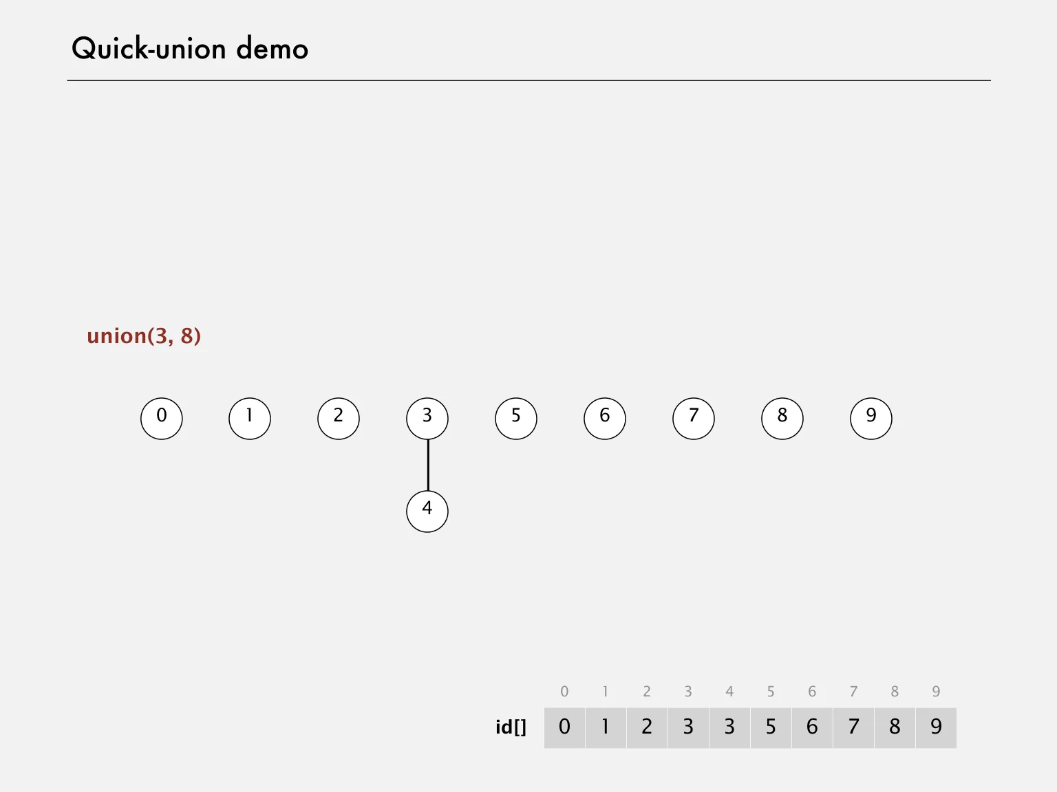
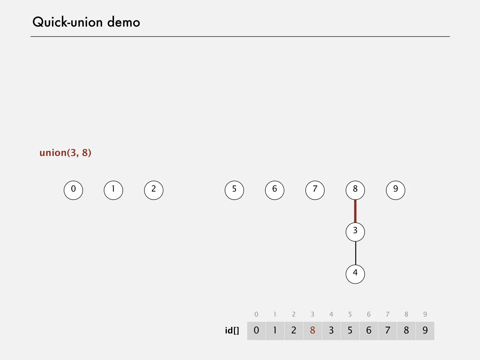
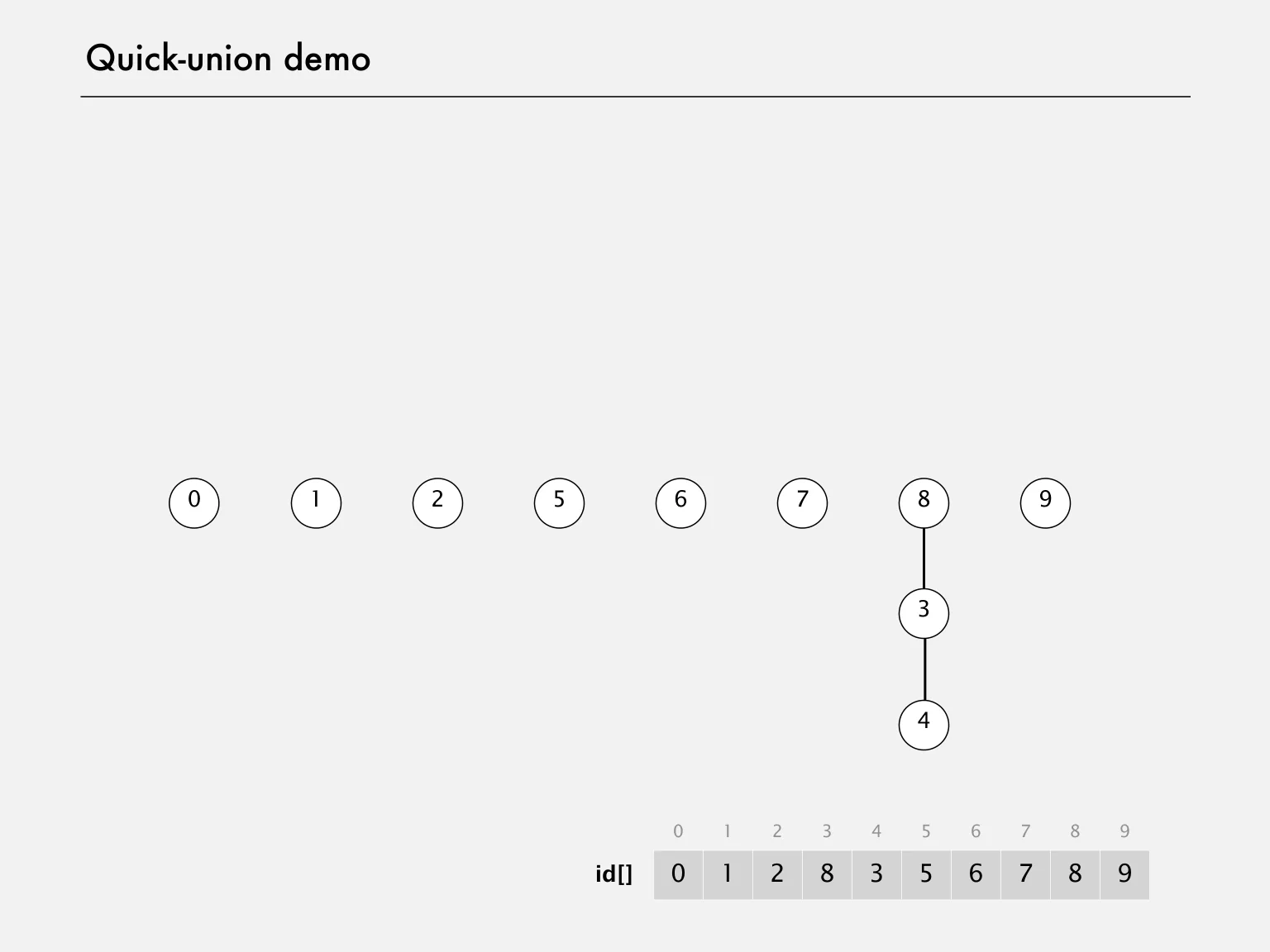
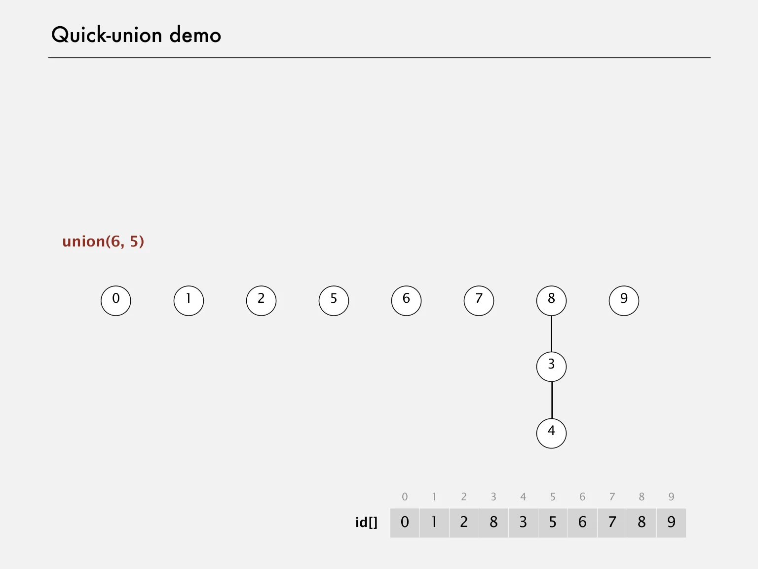
Trace quick-find and quick-union.
Explain the logarithmic height bound of weighted union.
Apply union–find to percolation.
Before you begin: Arrays · Trees and logarithms · Lecture 04: cost models
Expanded study guide
The dynamic connectivity problem
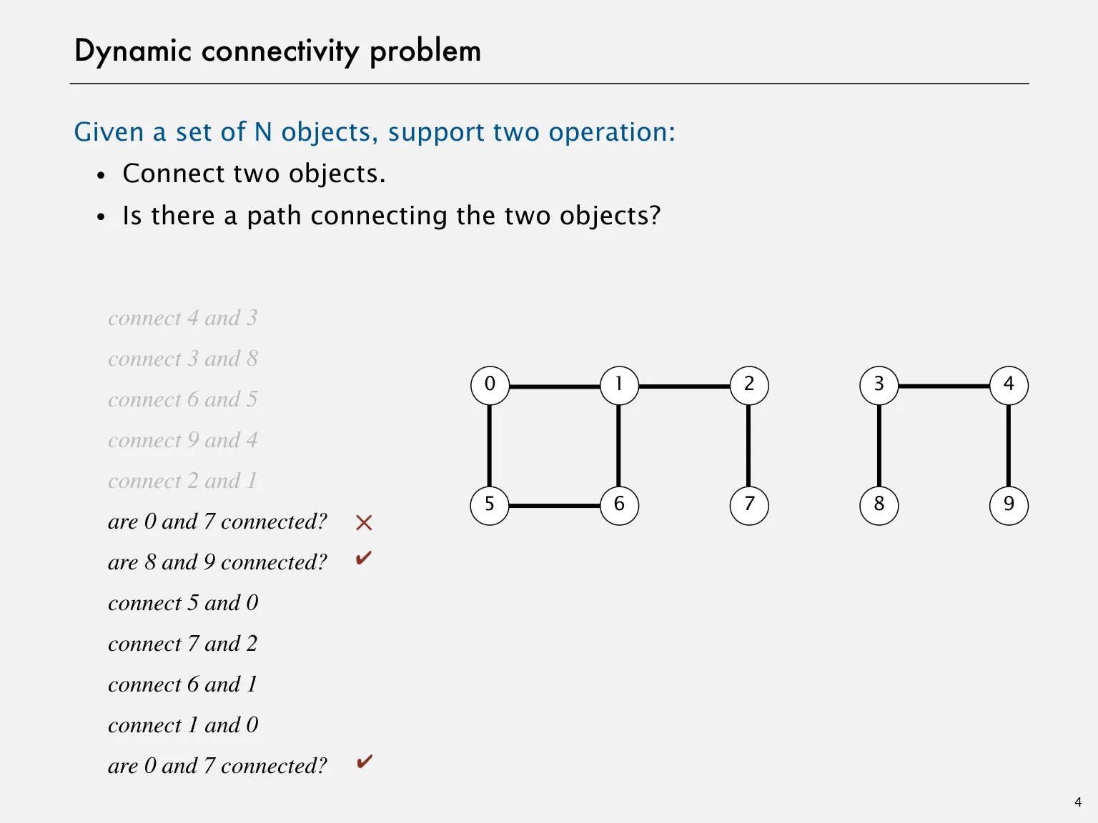
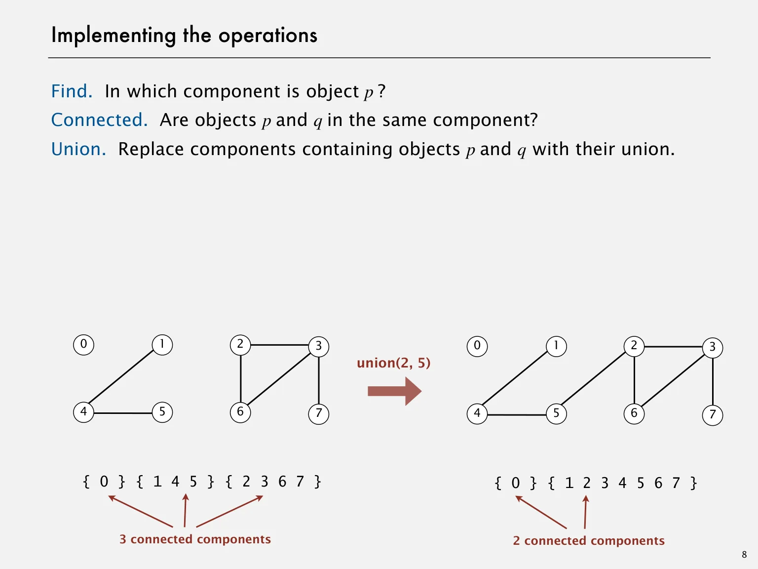
Maintain disjoint components of objects numbered 0 through n−1. A union operation joins two components, and a find operation identifies the component containing an object. Two objects are connected when their representatives agree.
Connectivity is reflexive, symmetric and transitive, so it partitions the objects into equivalence classes. We need component membership, not a list of every path connecting two objects.
Quick-find: eager labels
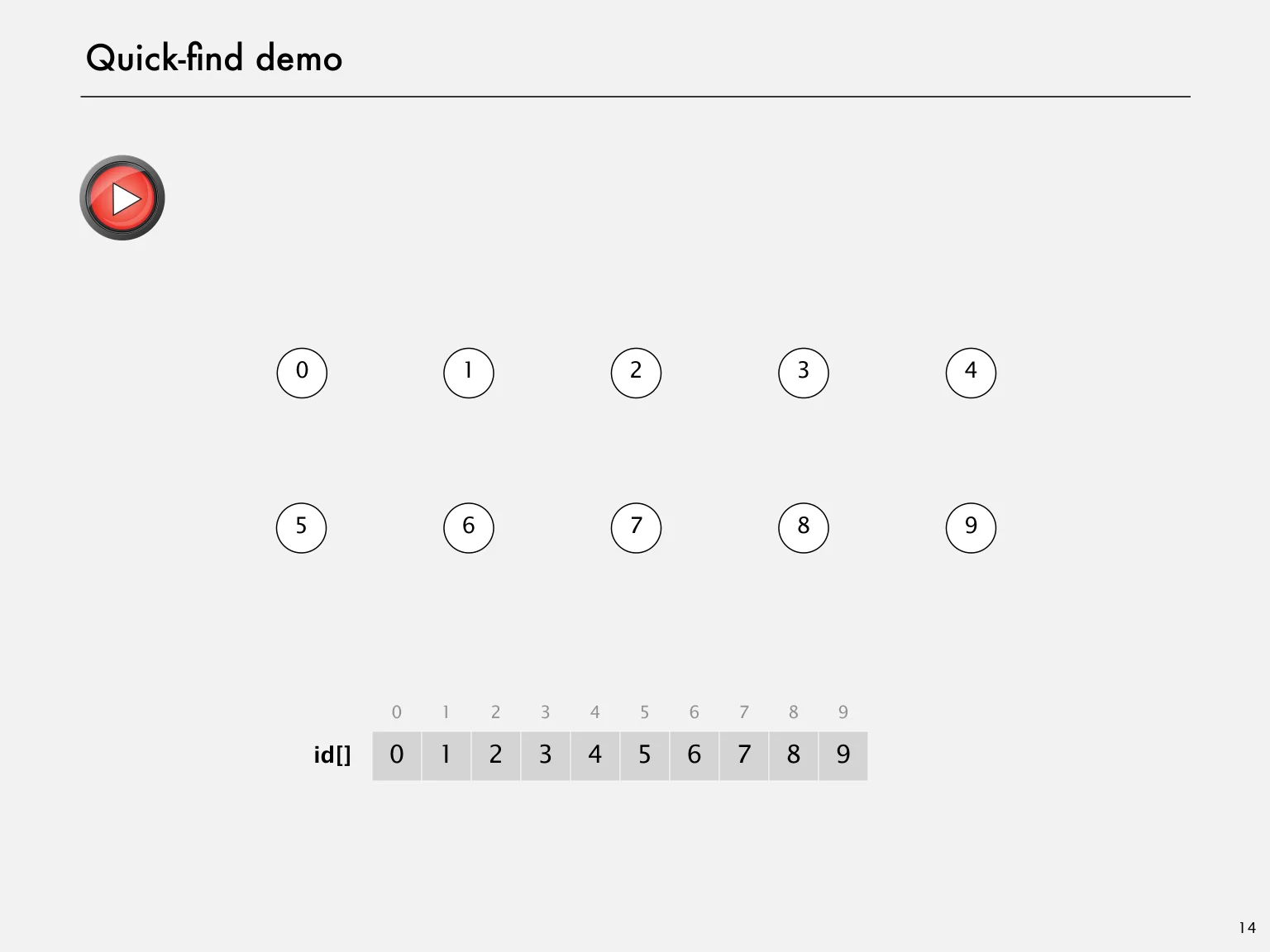
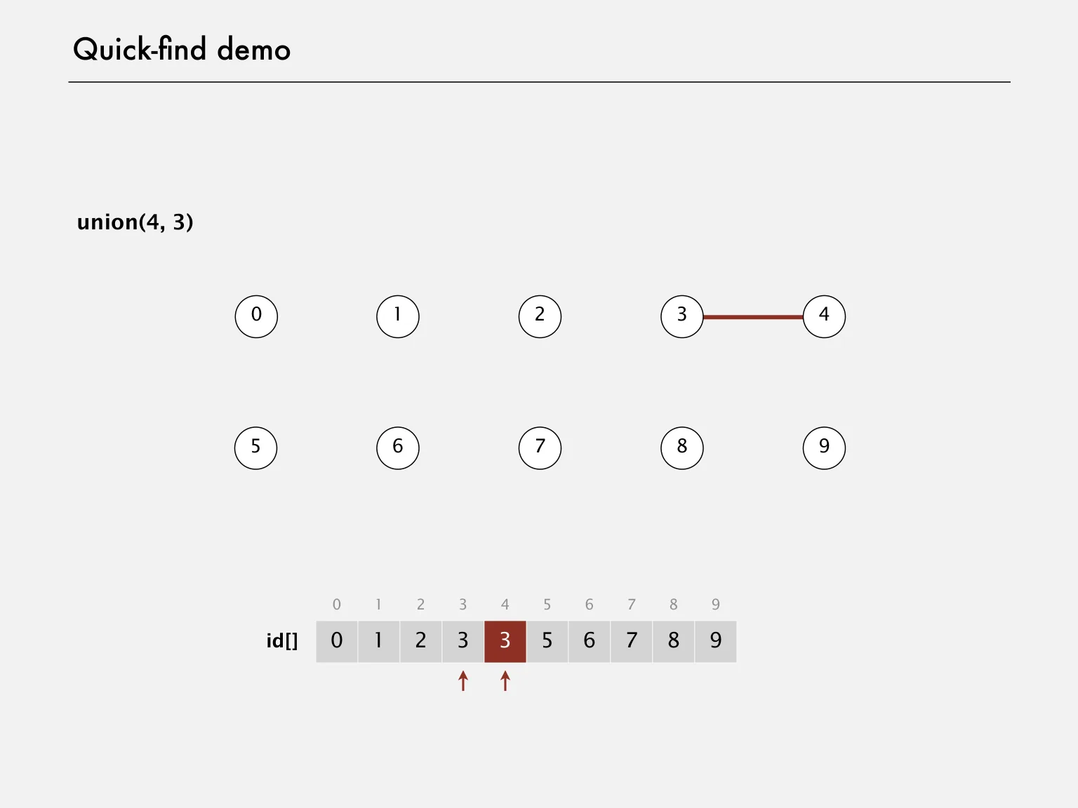
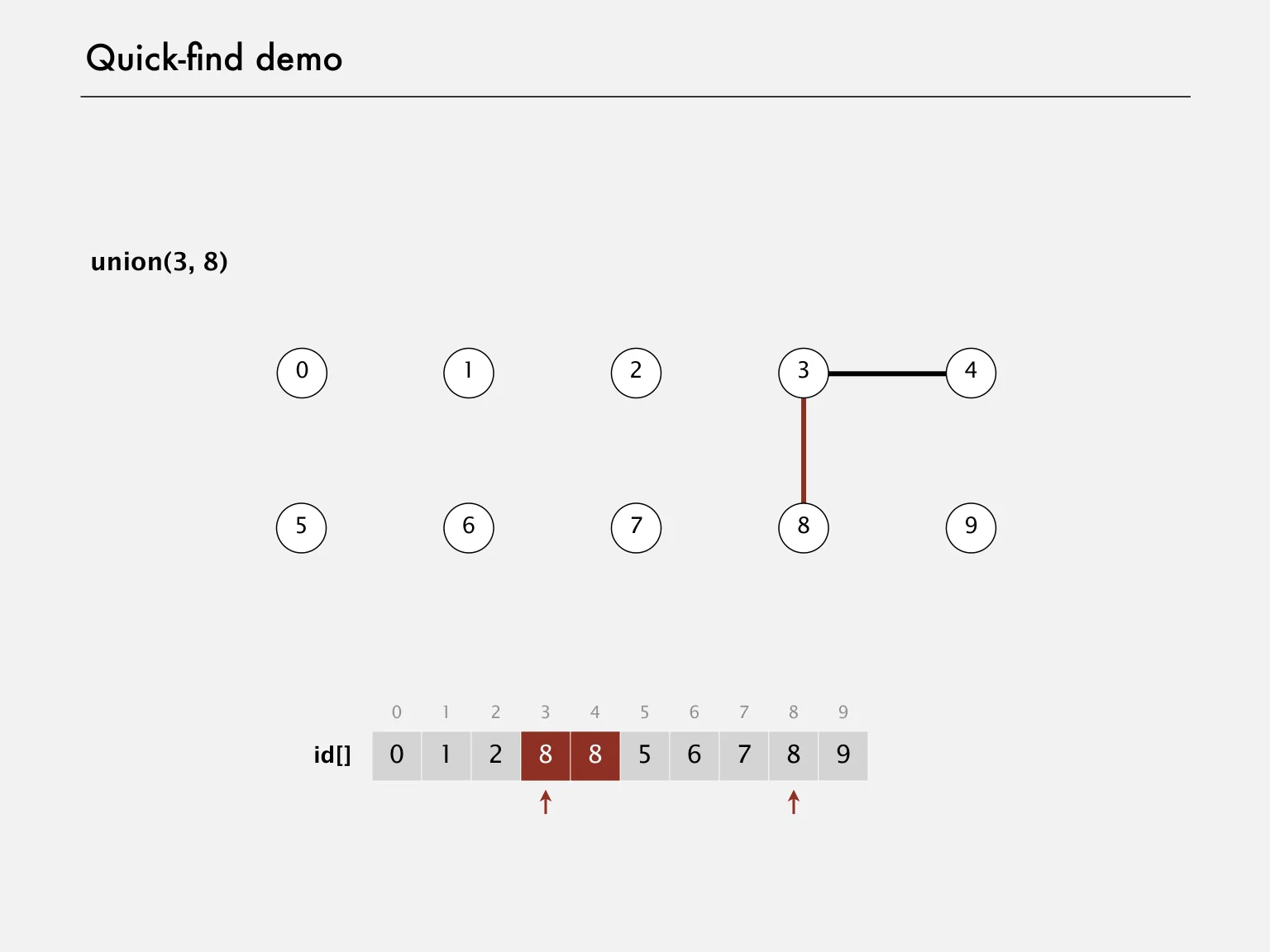
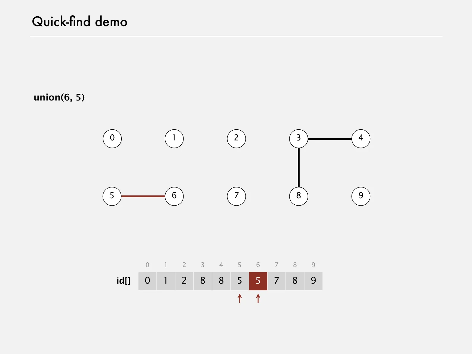
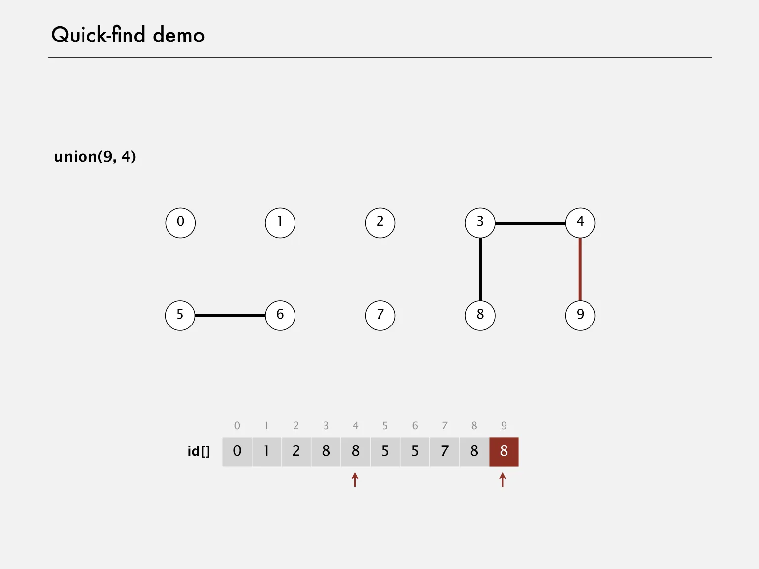
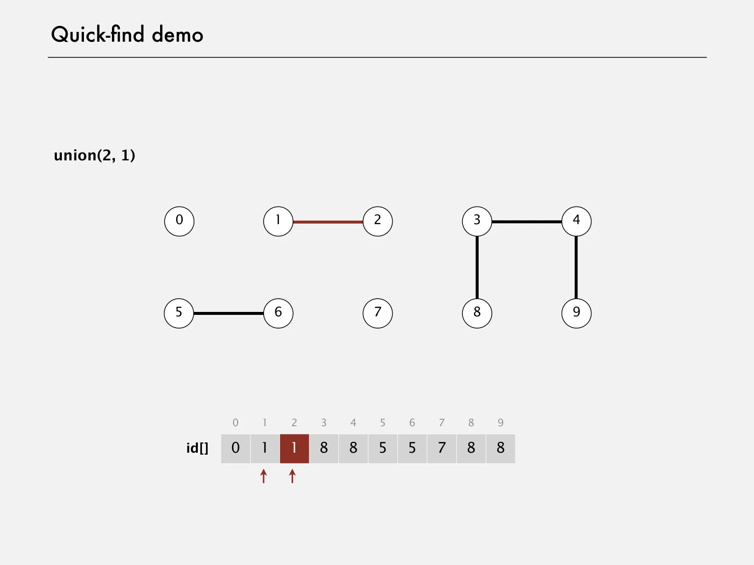
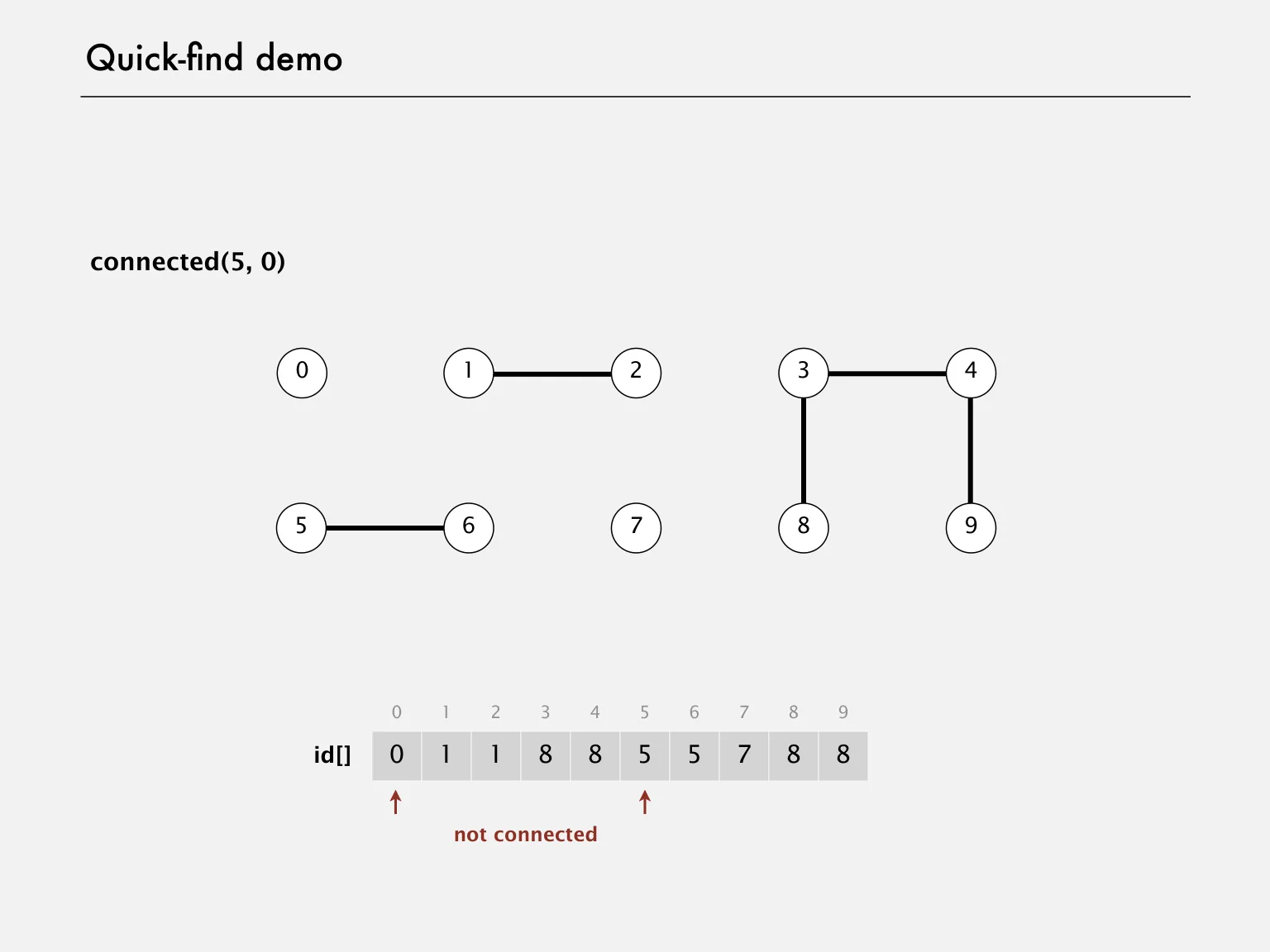
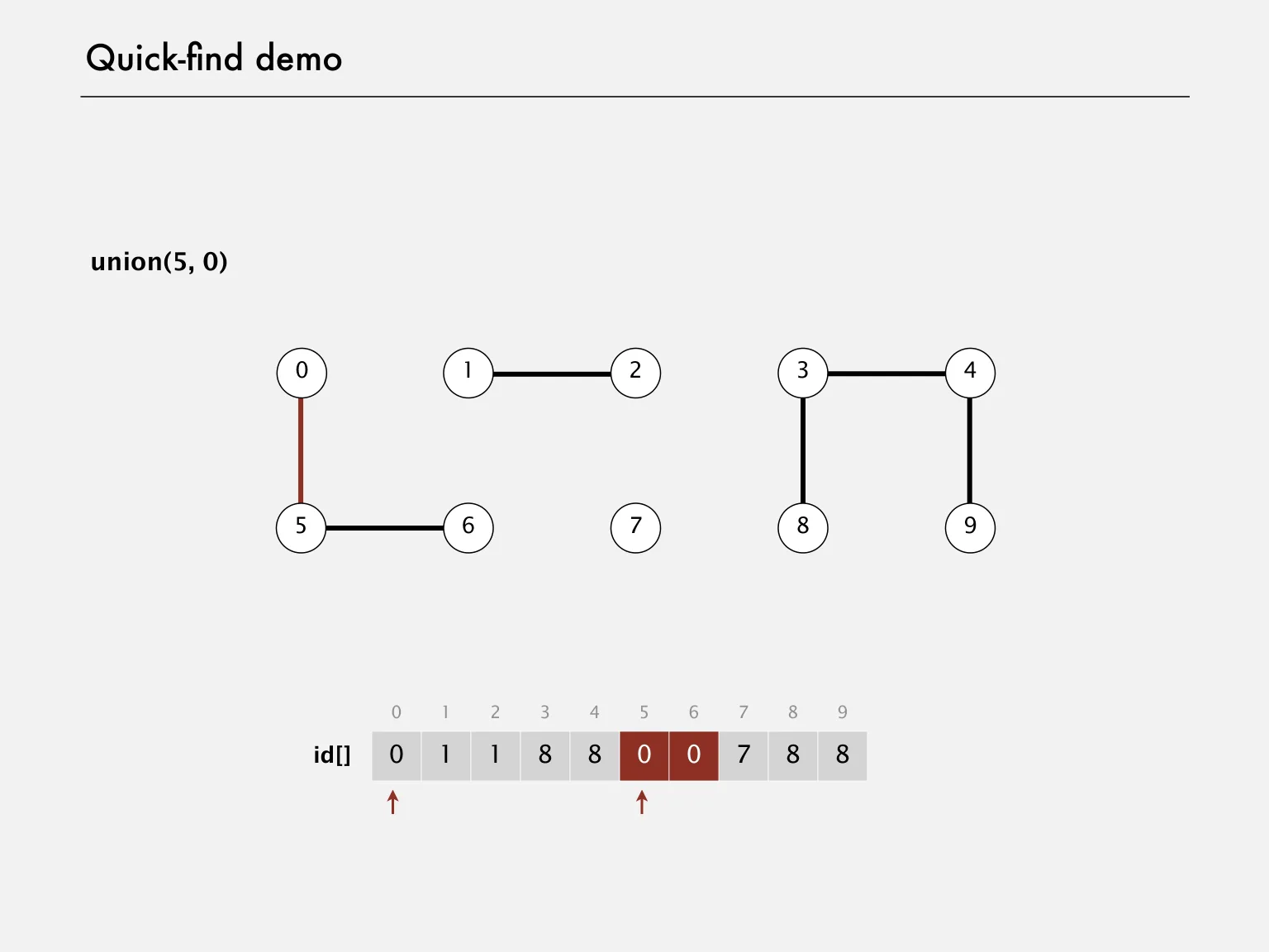
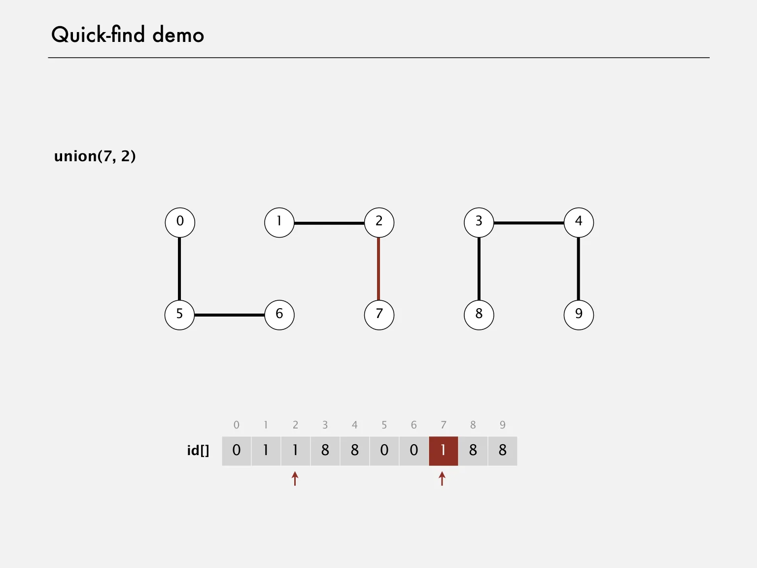
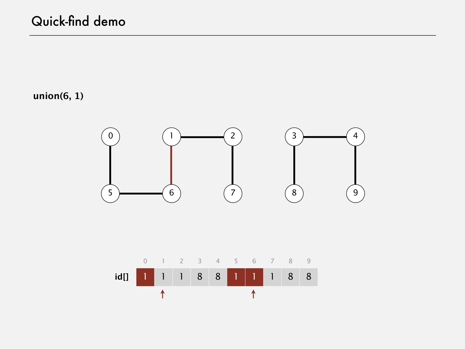
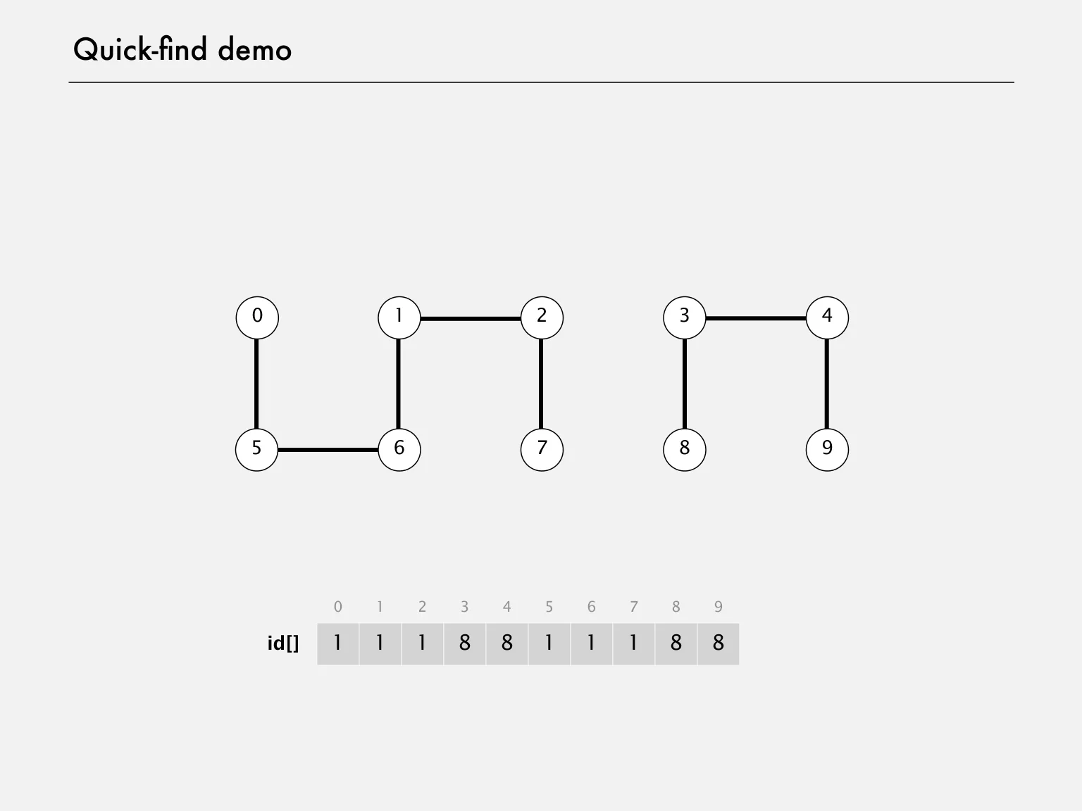
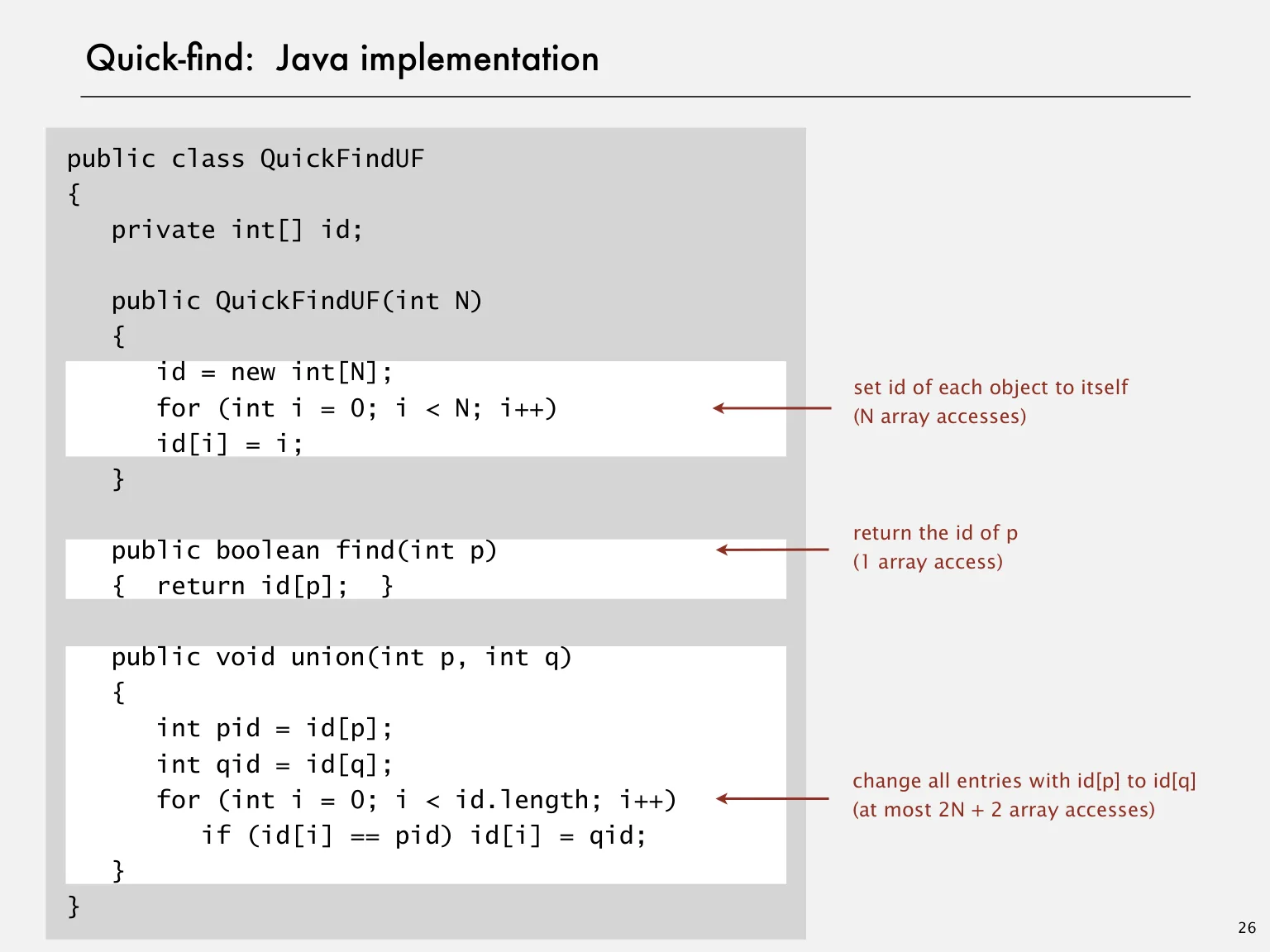
Store a component identifier in id[p] for every object p. Find reads one entry. To union p and q, save both original labels and scan the entire array, changing entries matching p’s old label to q’s label.
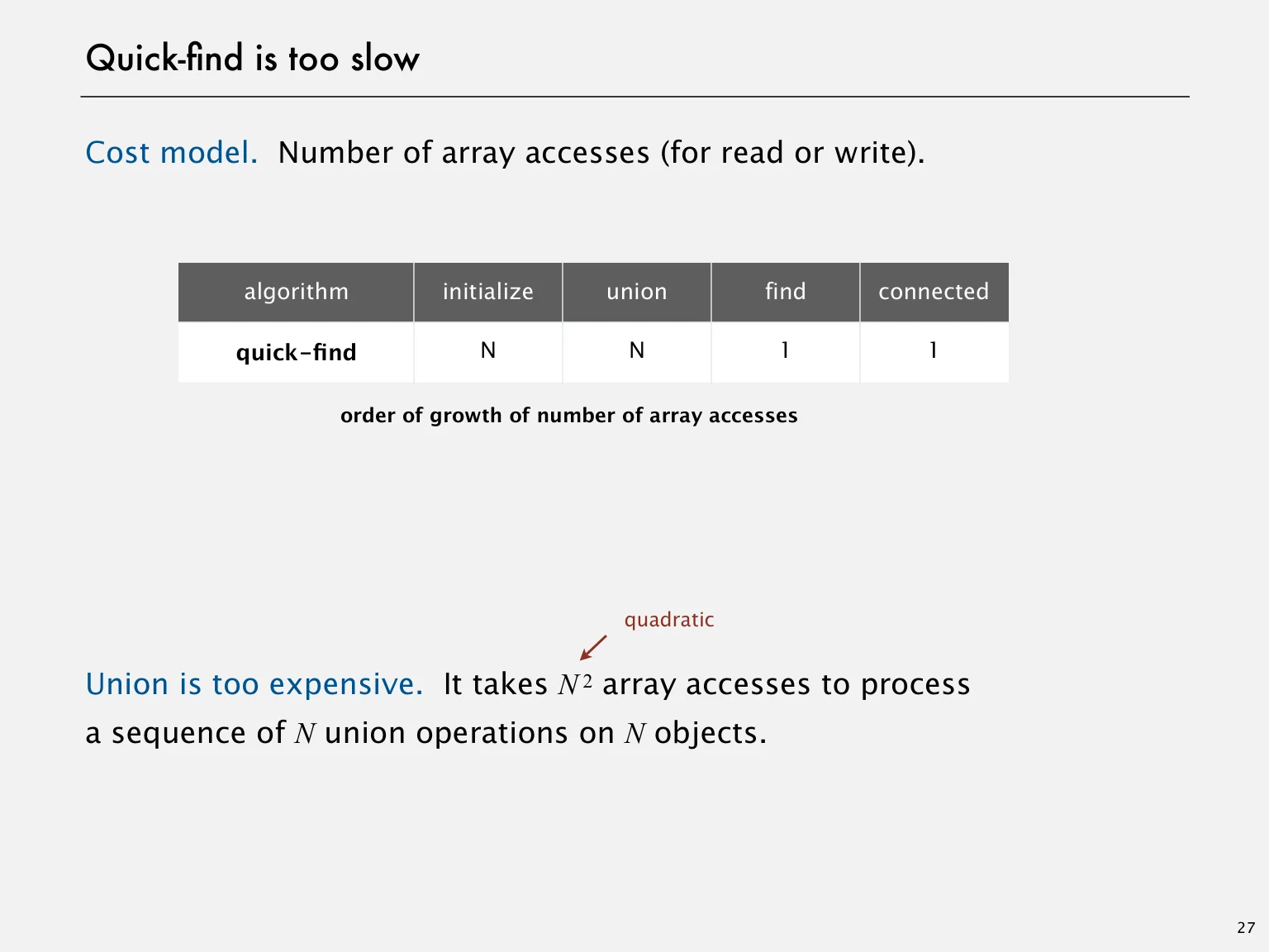
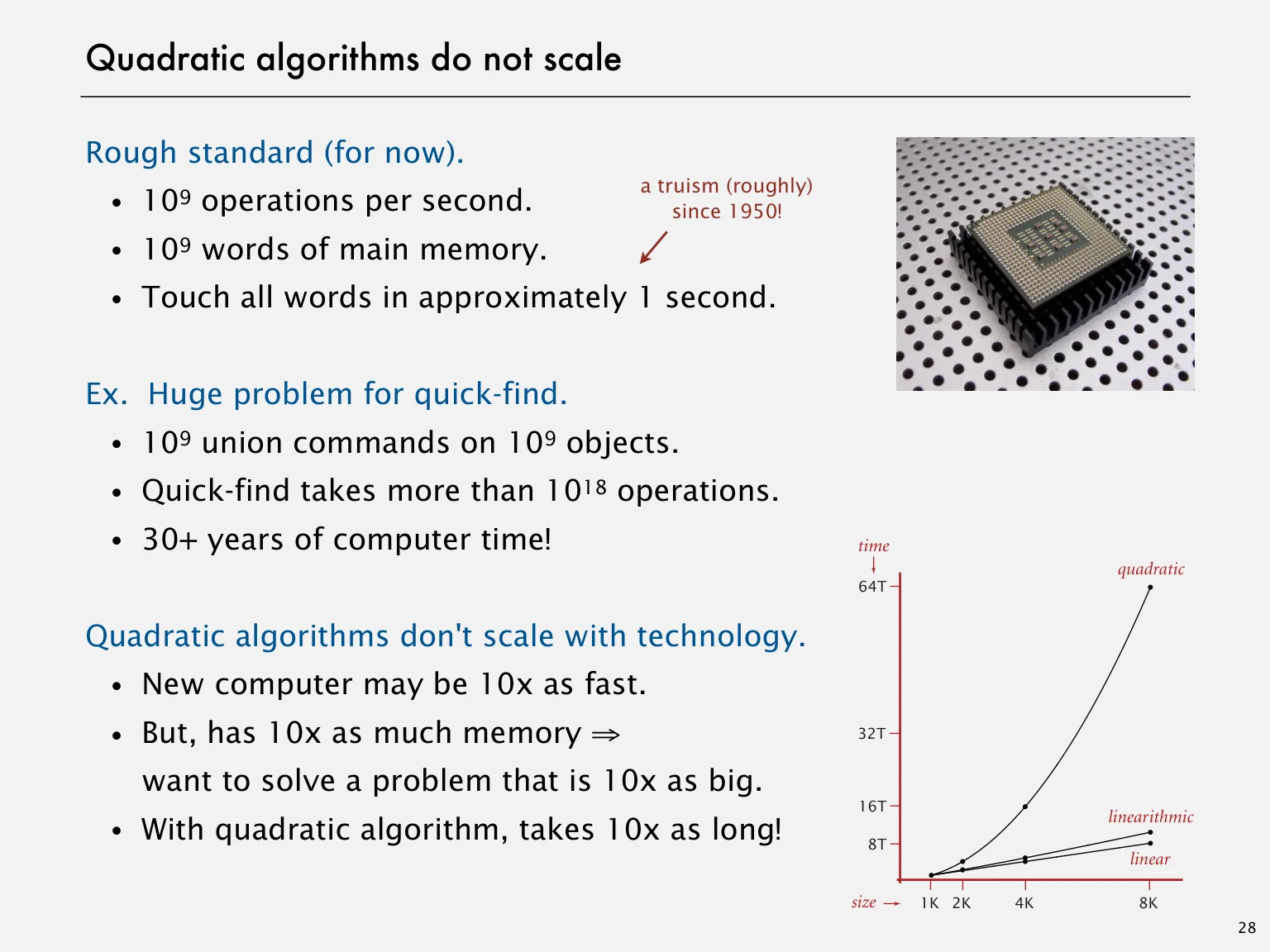
A find is Θ(1), while a union that scans the array is Θ(n). A sequence of n such unions can therefore require Θ(n²) work. Saving the old label before changing entries is essential for a correct update.
Initial state for five objects: [0, 1, 2, 3, 4].
union(0, 1): [1, 1, 2, 3, 4].
union(1, 2): [2, 2, 2, 3, 4].
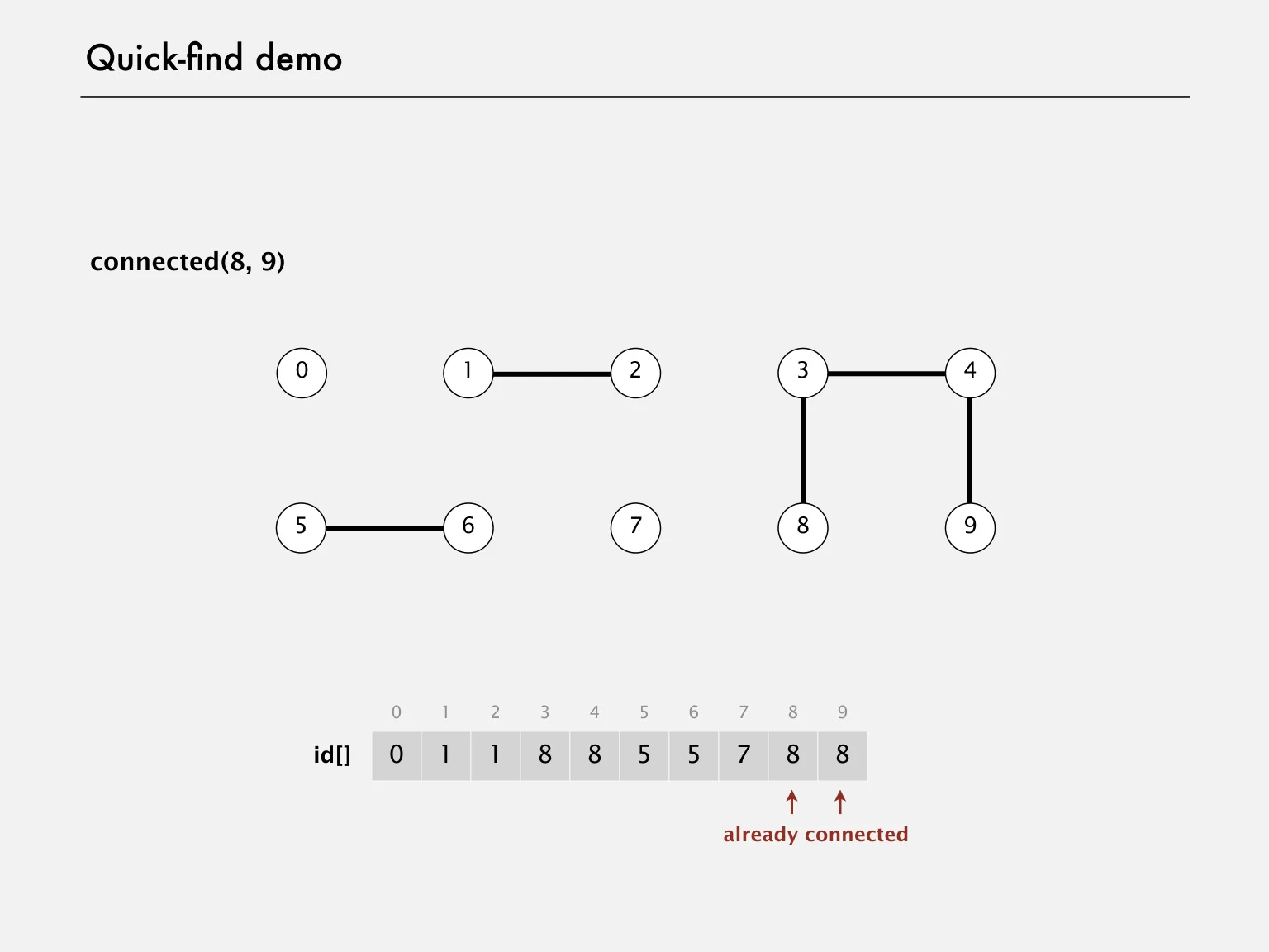
connected(0, 2) is true because both labels are 2.
Quick-union: parent-pointer forests
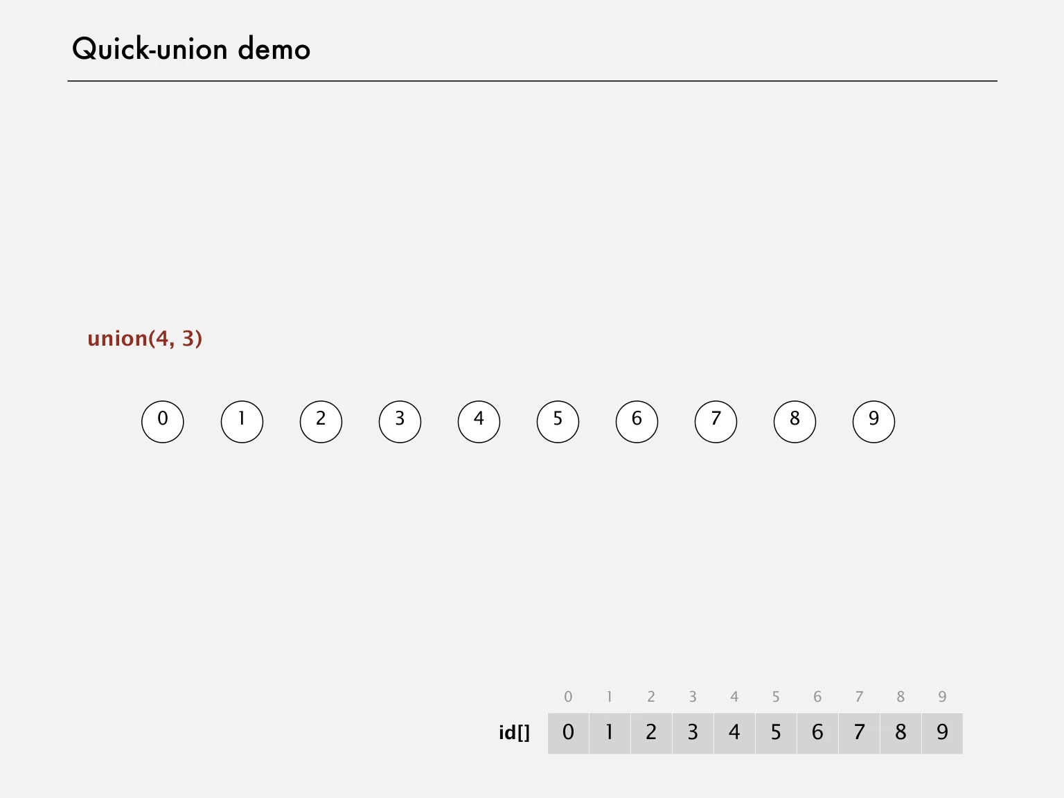
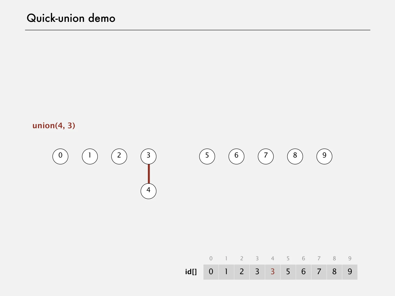
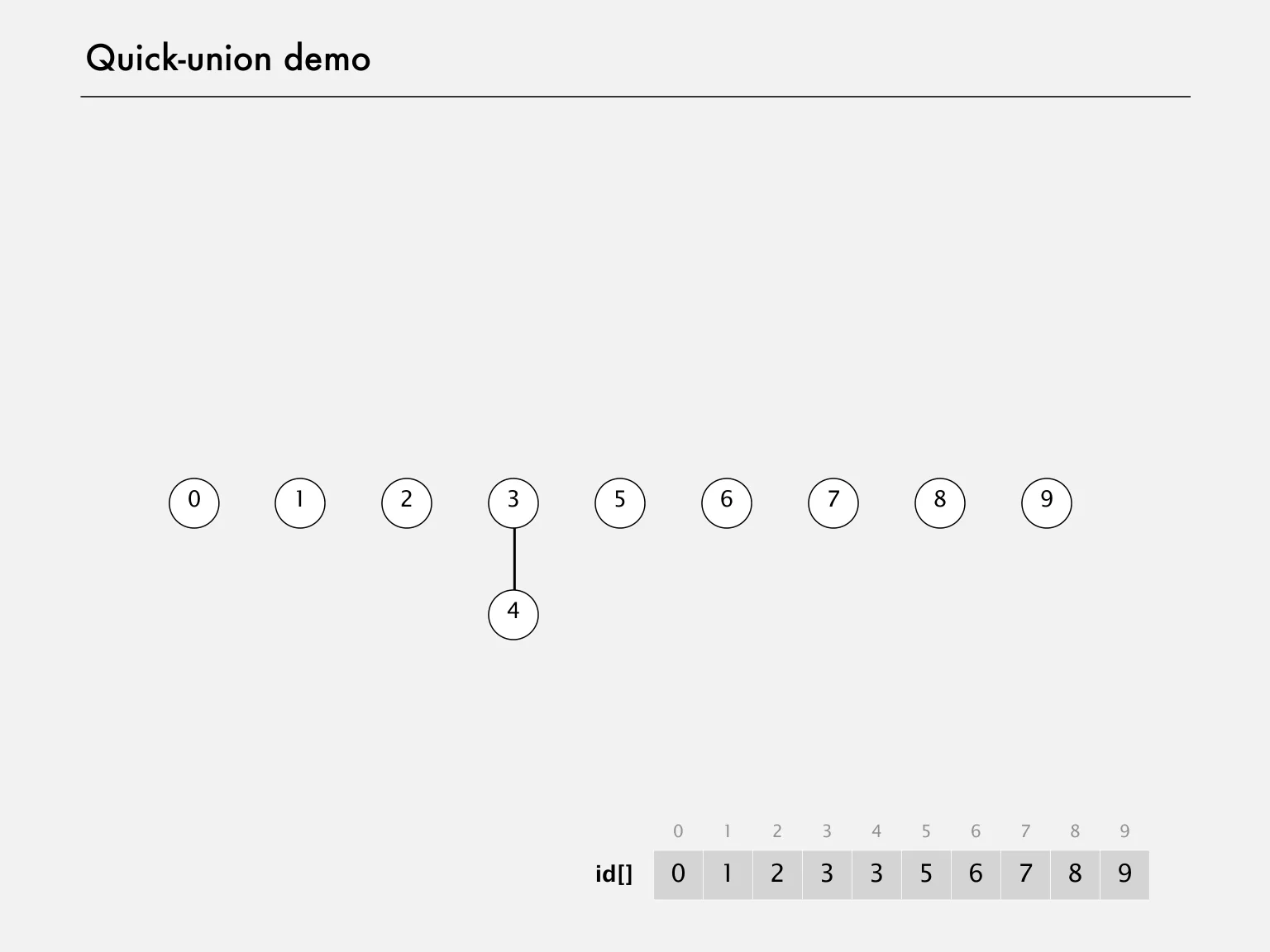
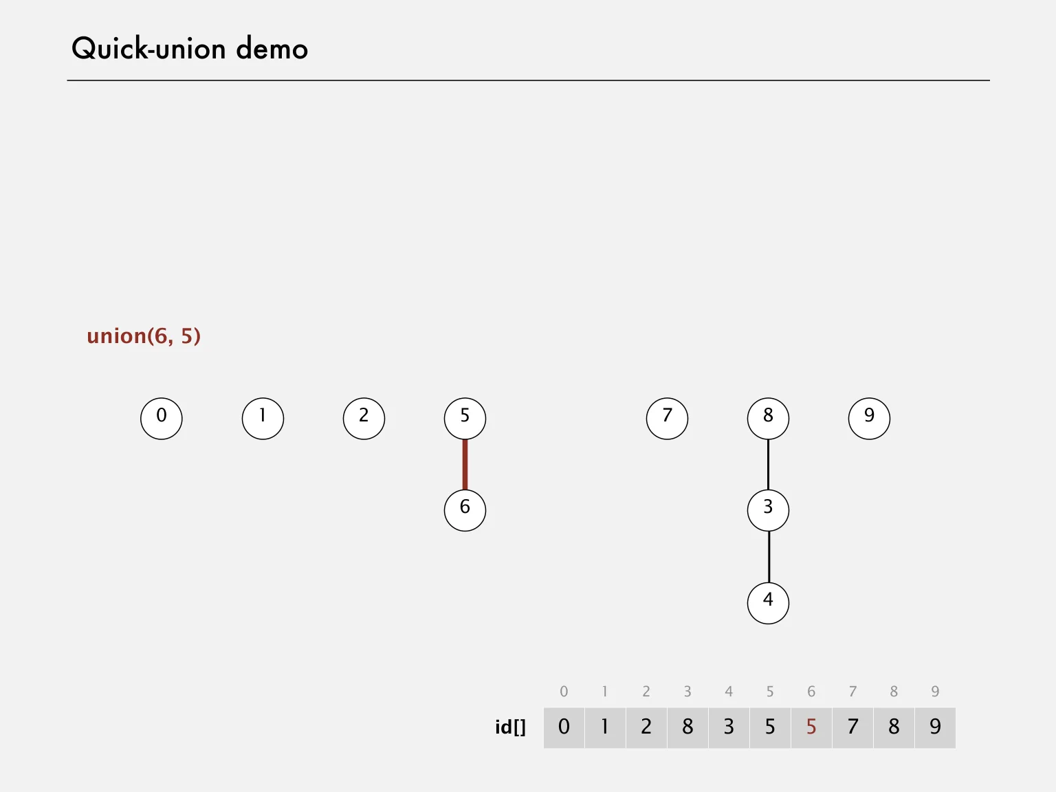
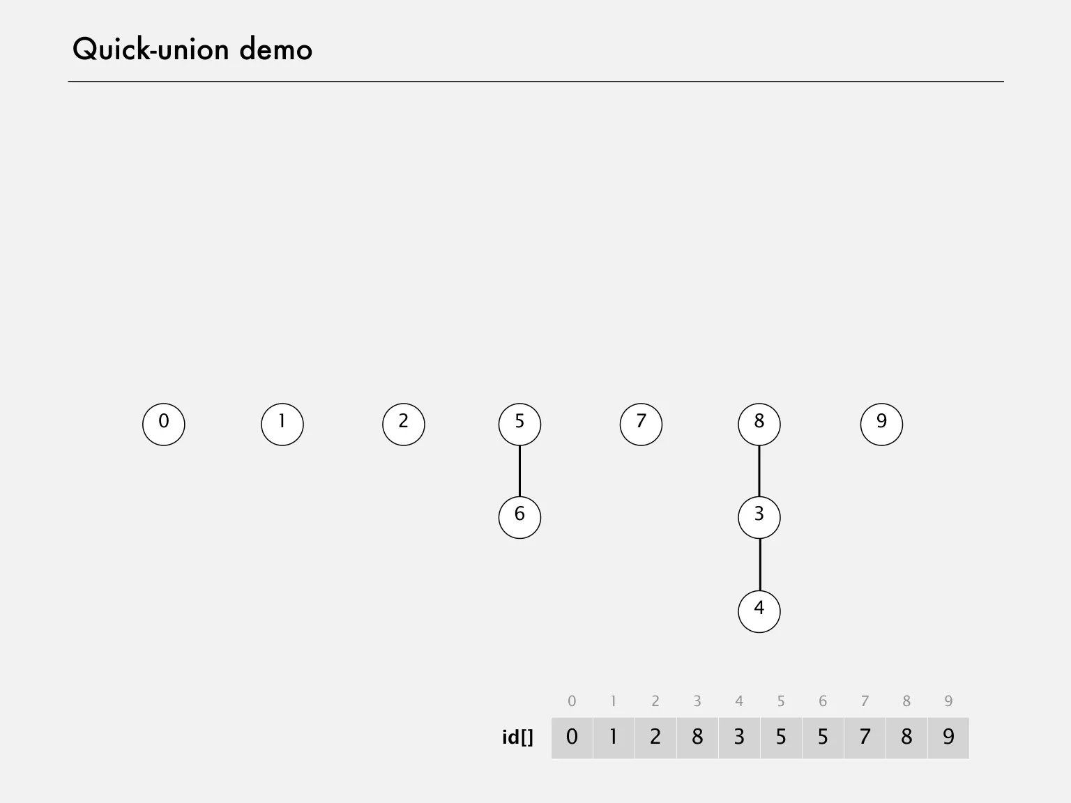
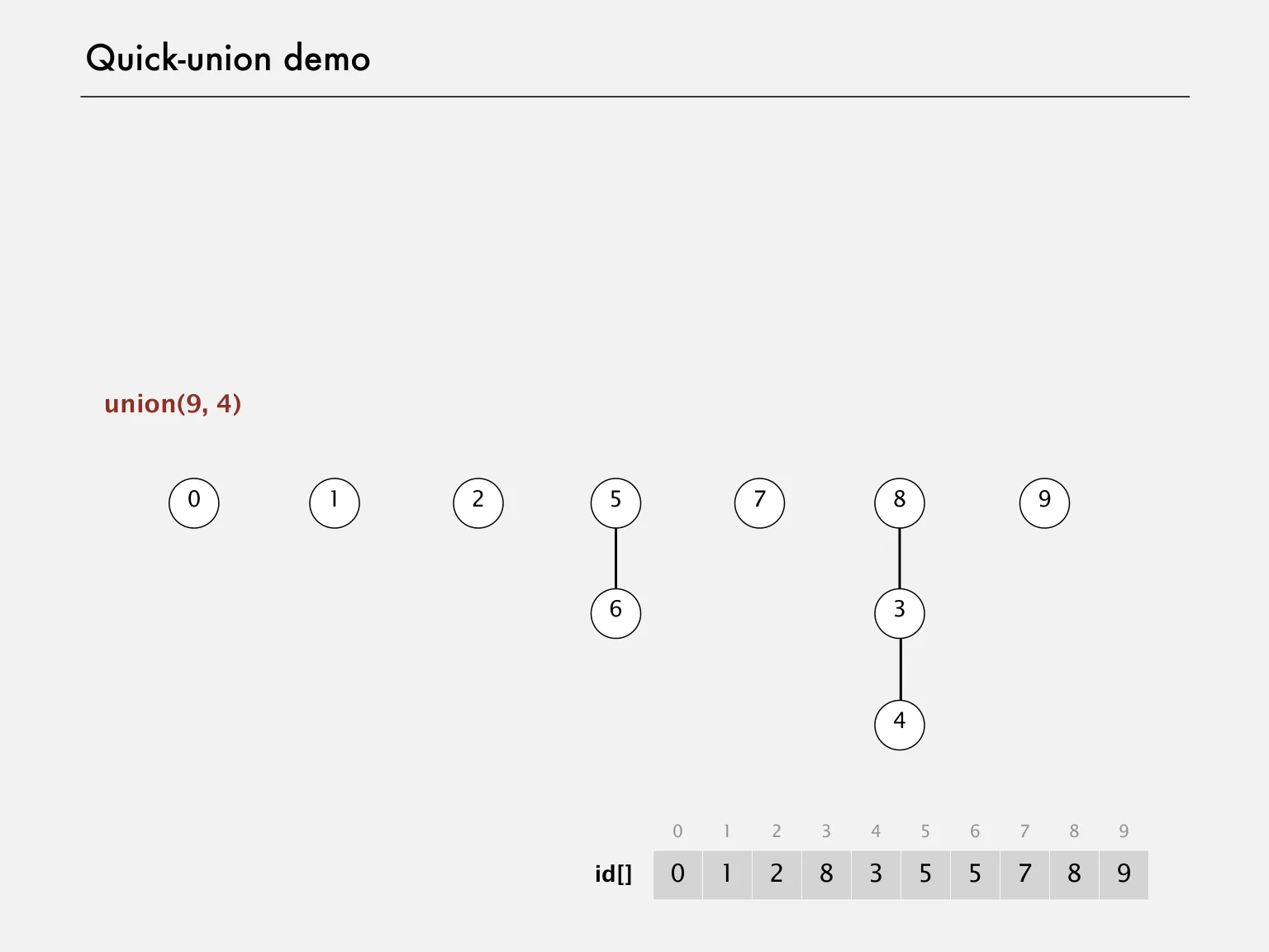
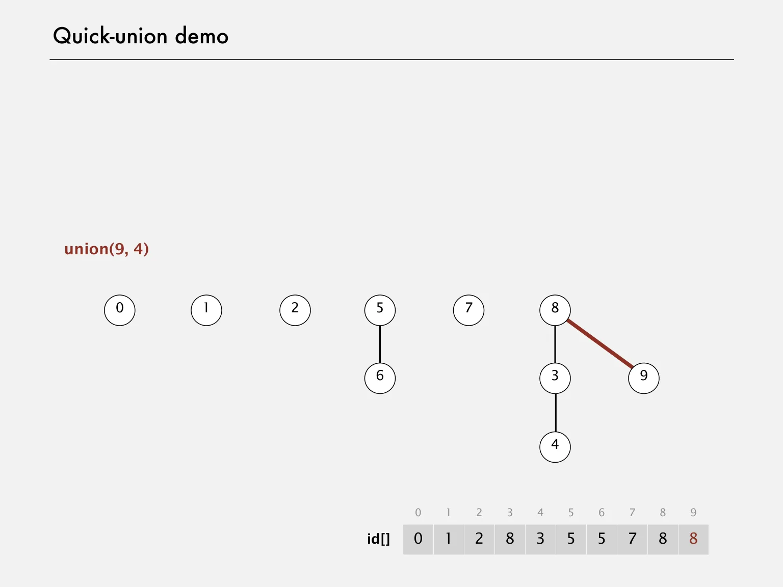
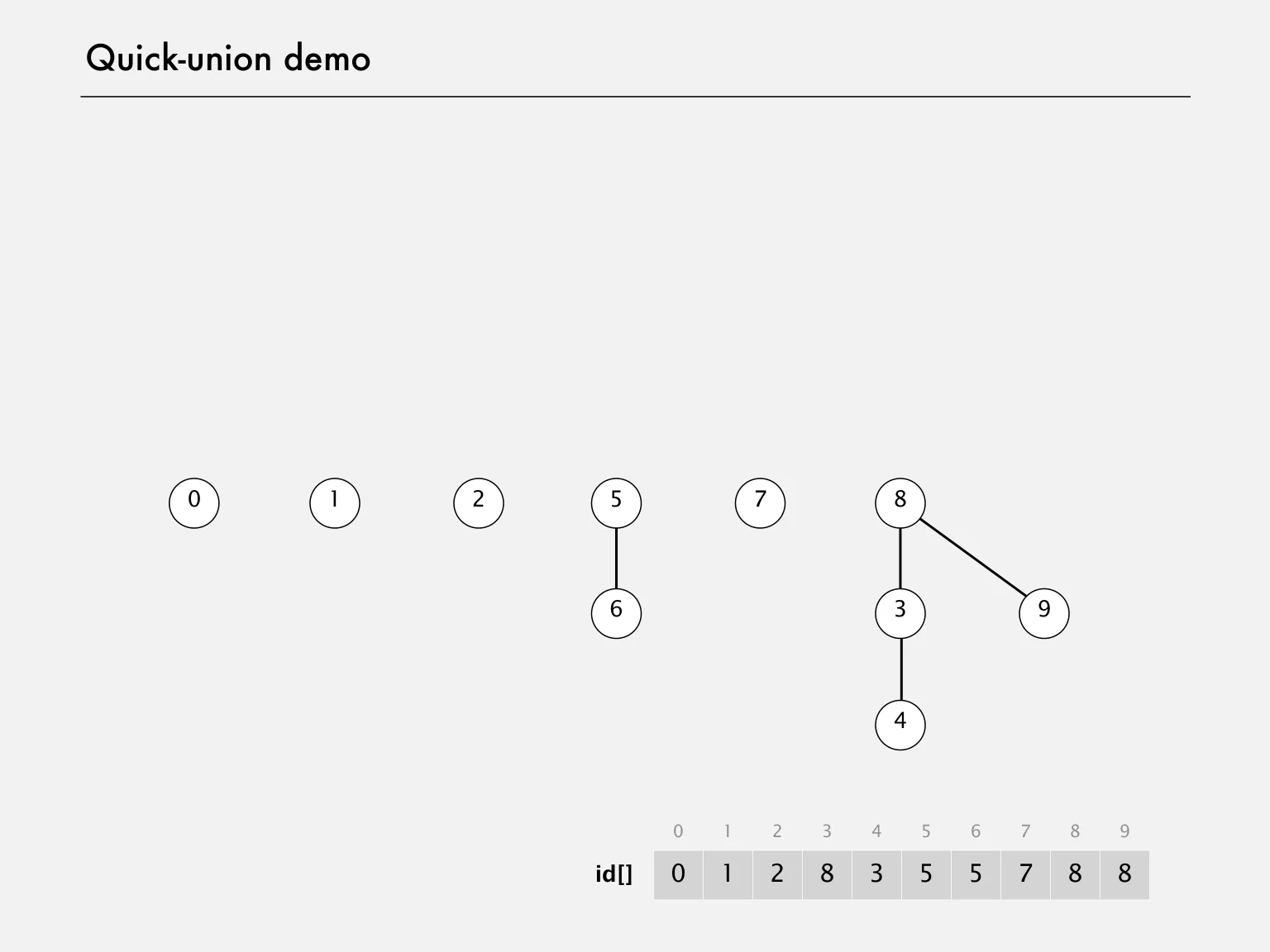
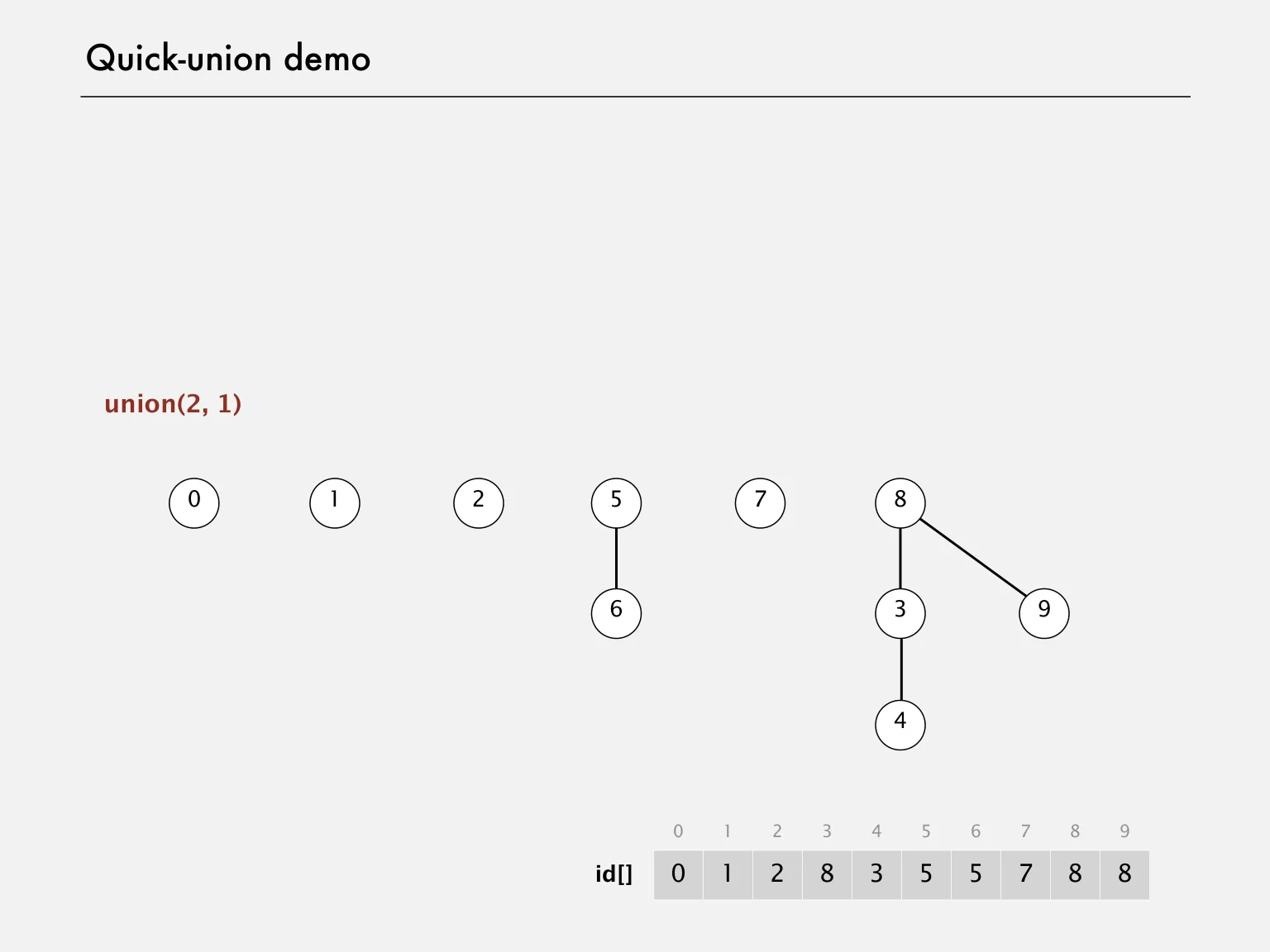
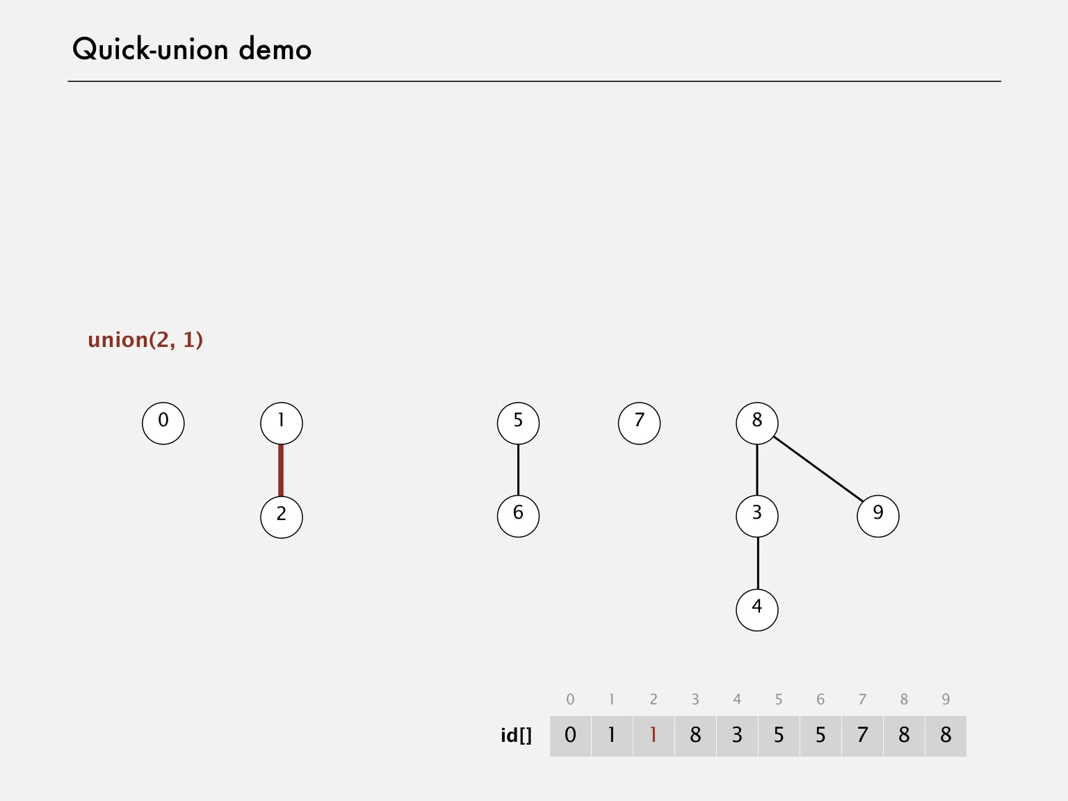
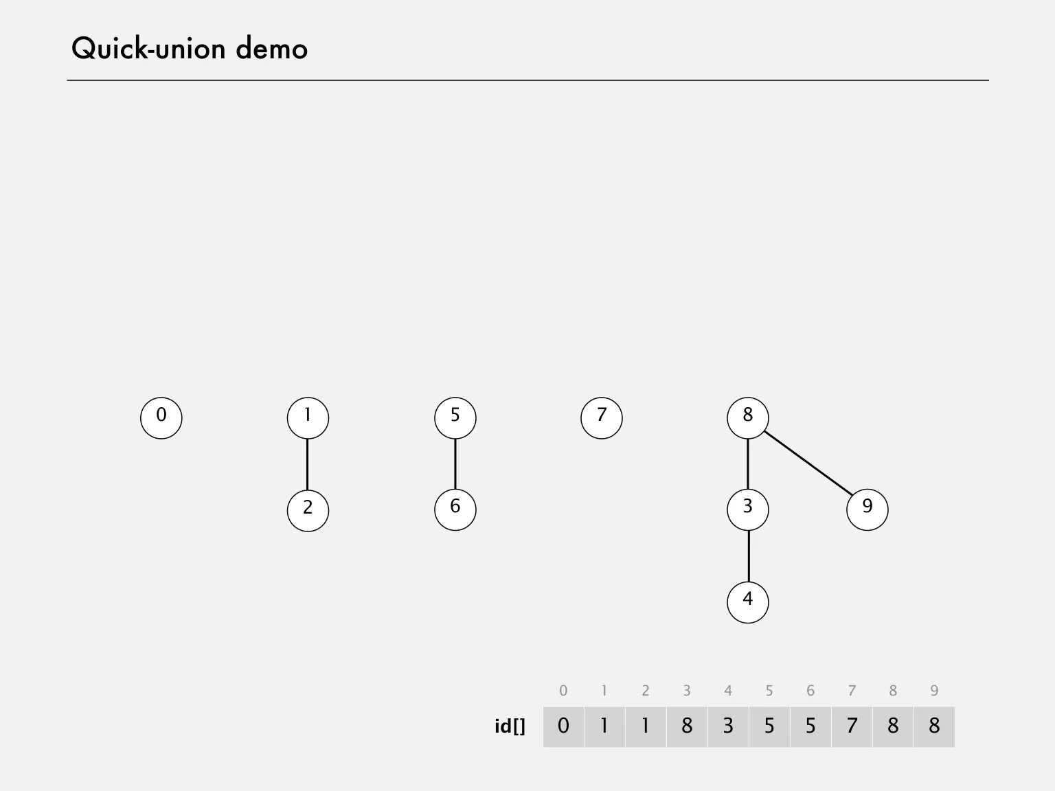
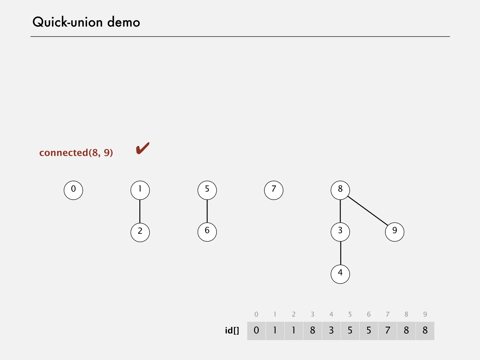
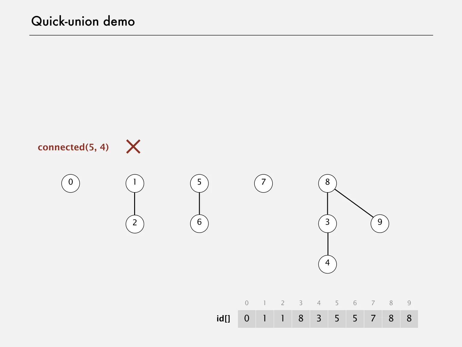
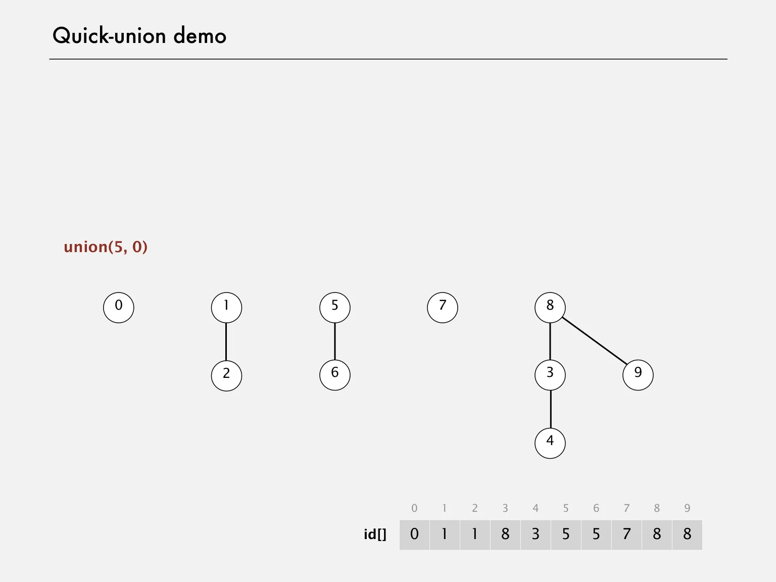
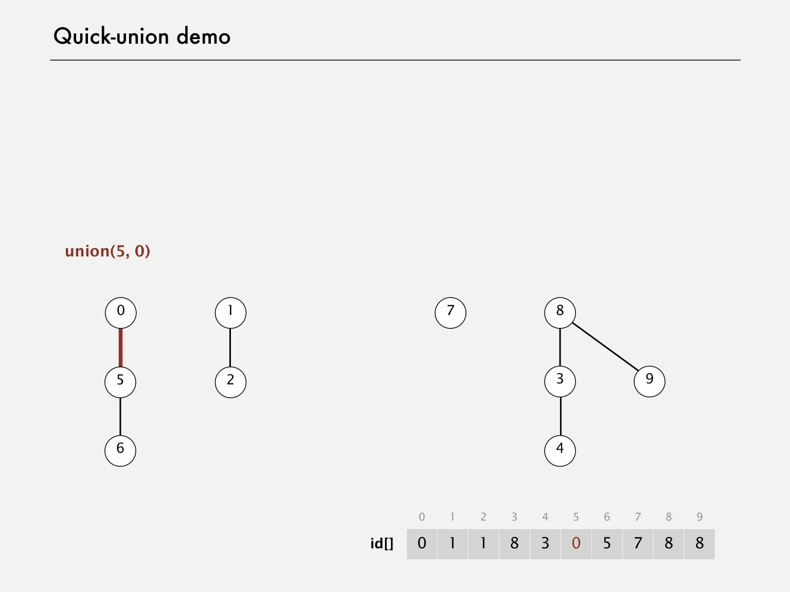
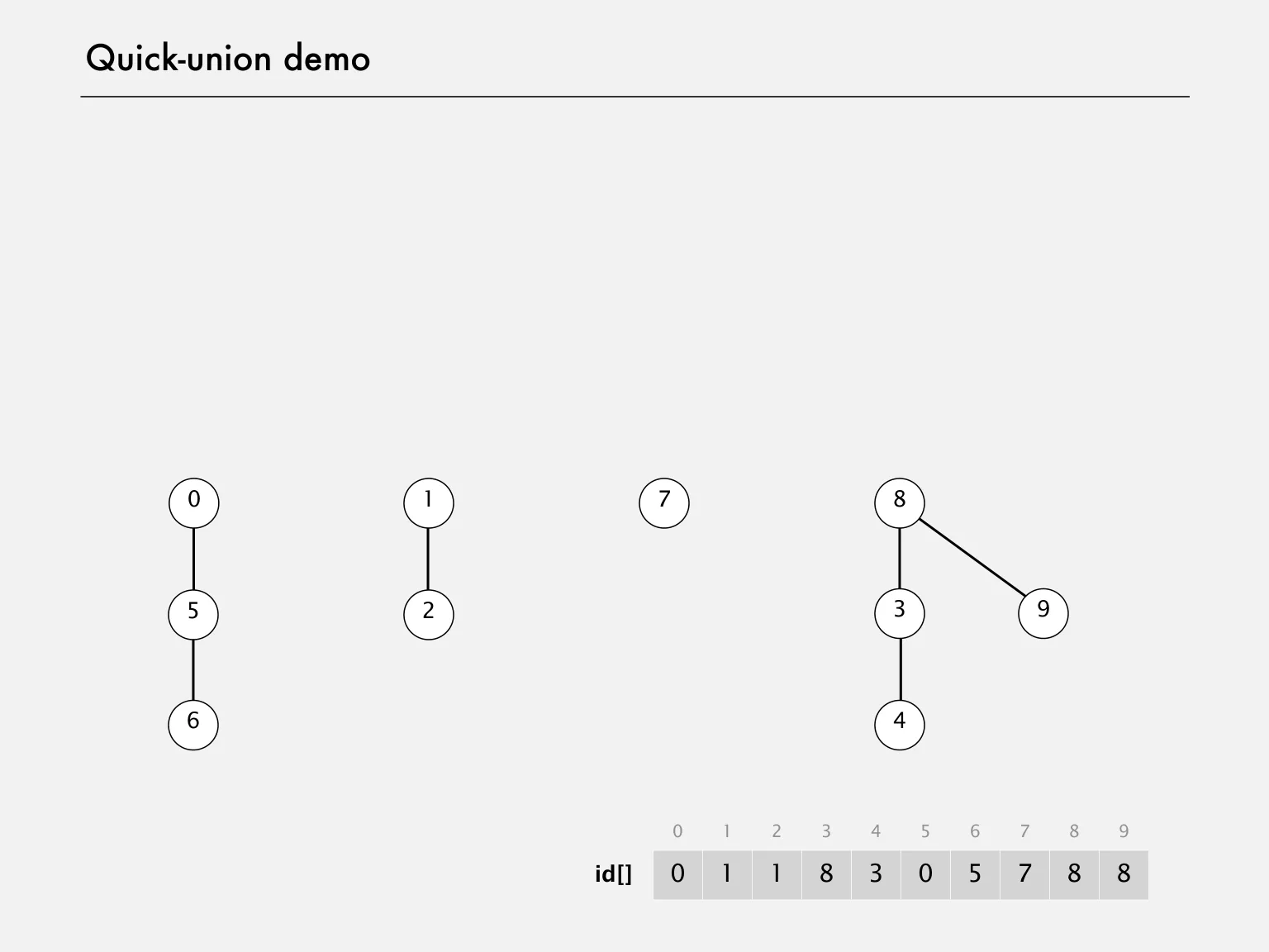
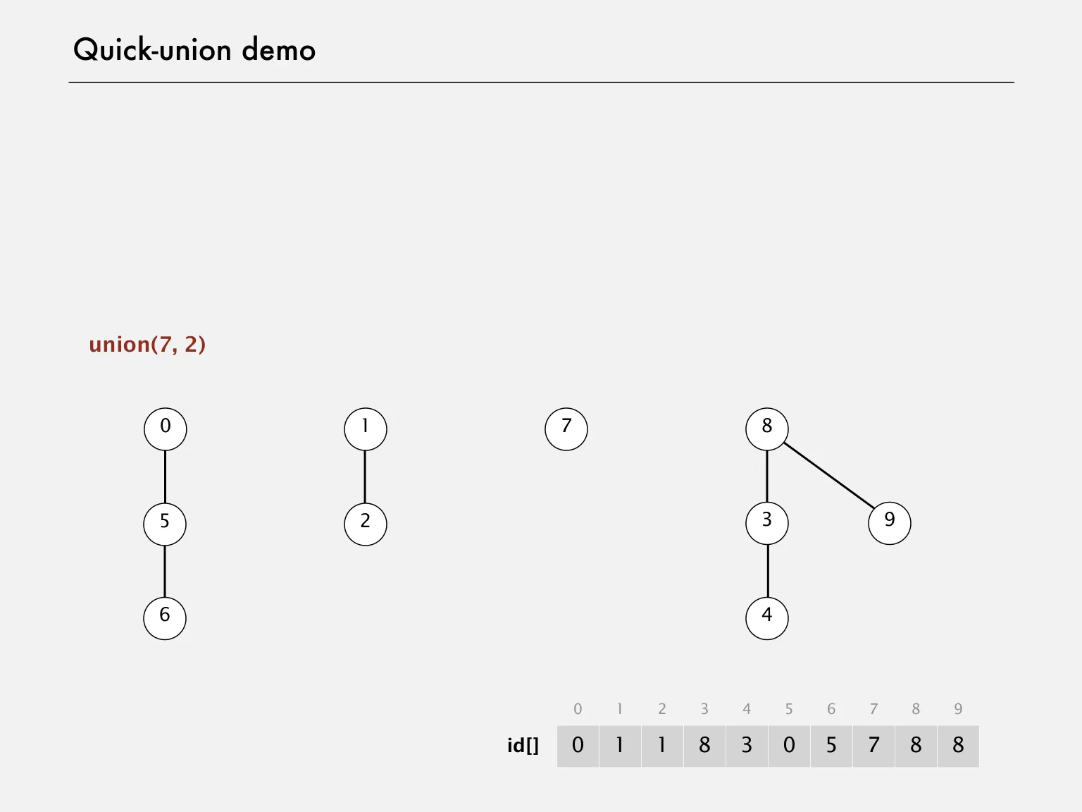
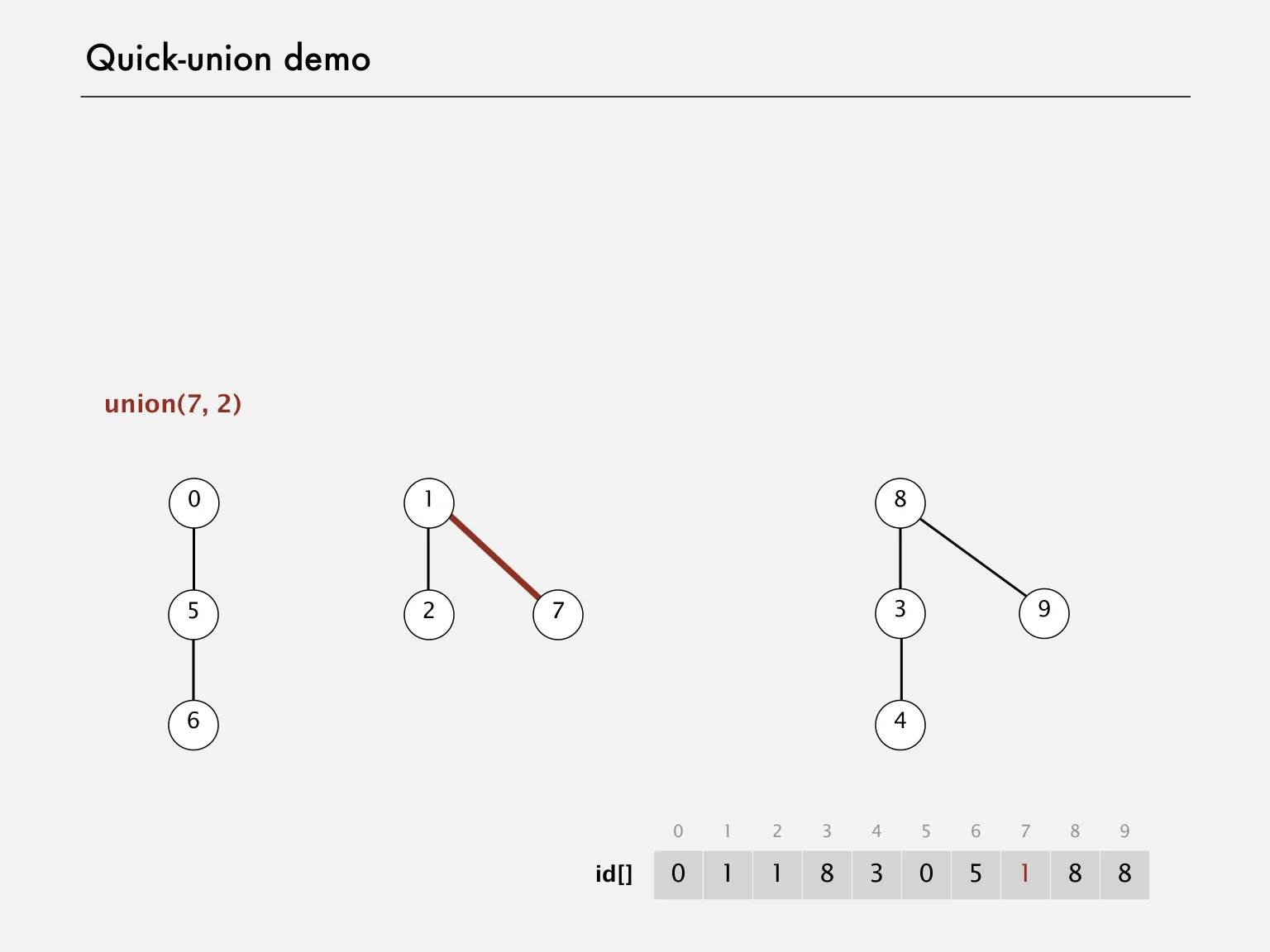
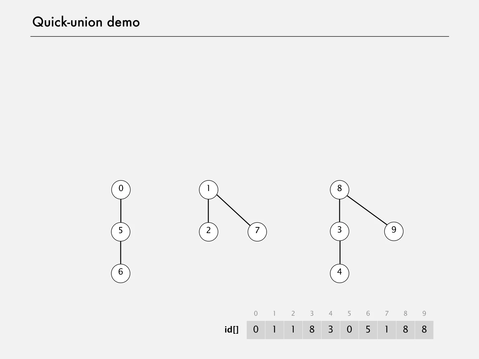
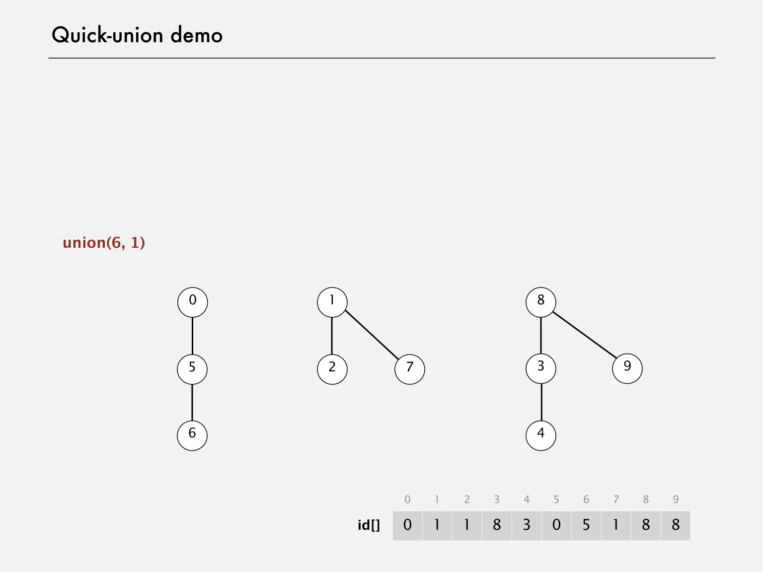
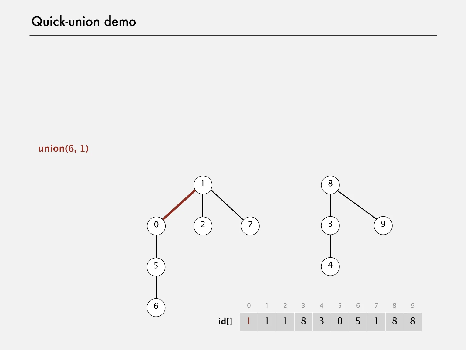
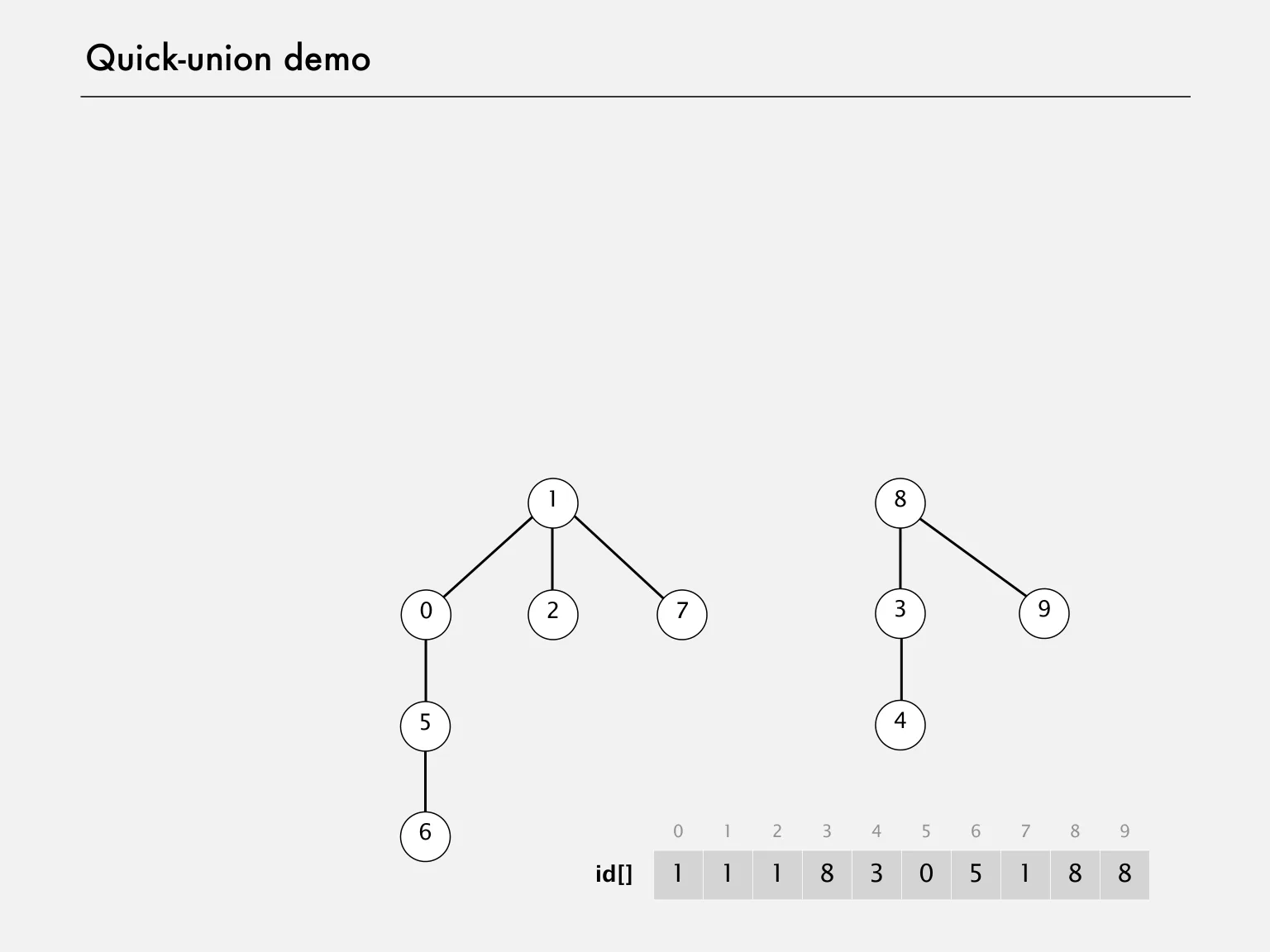
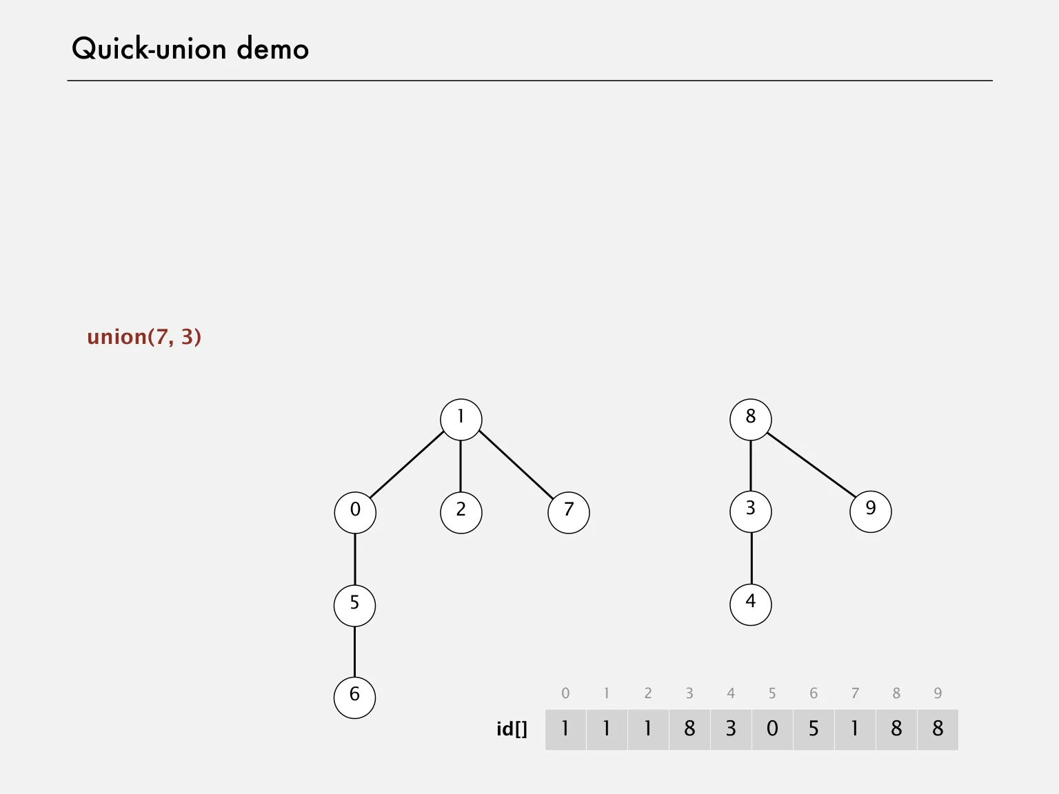
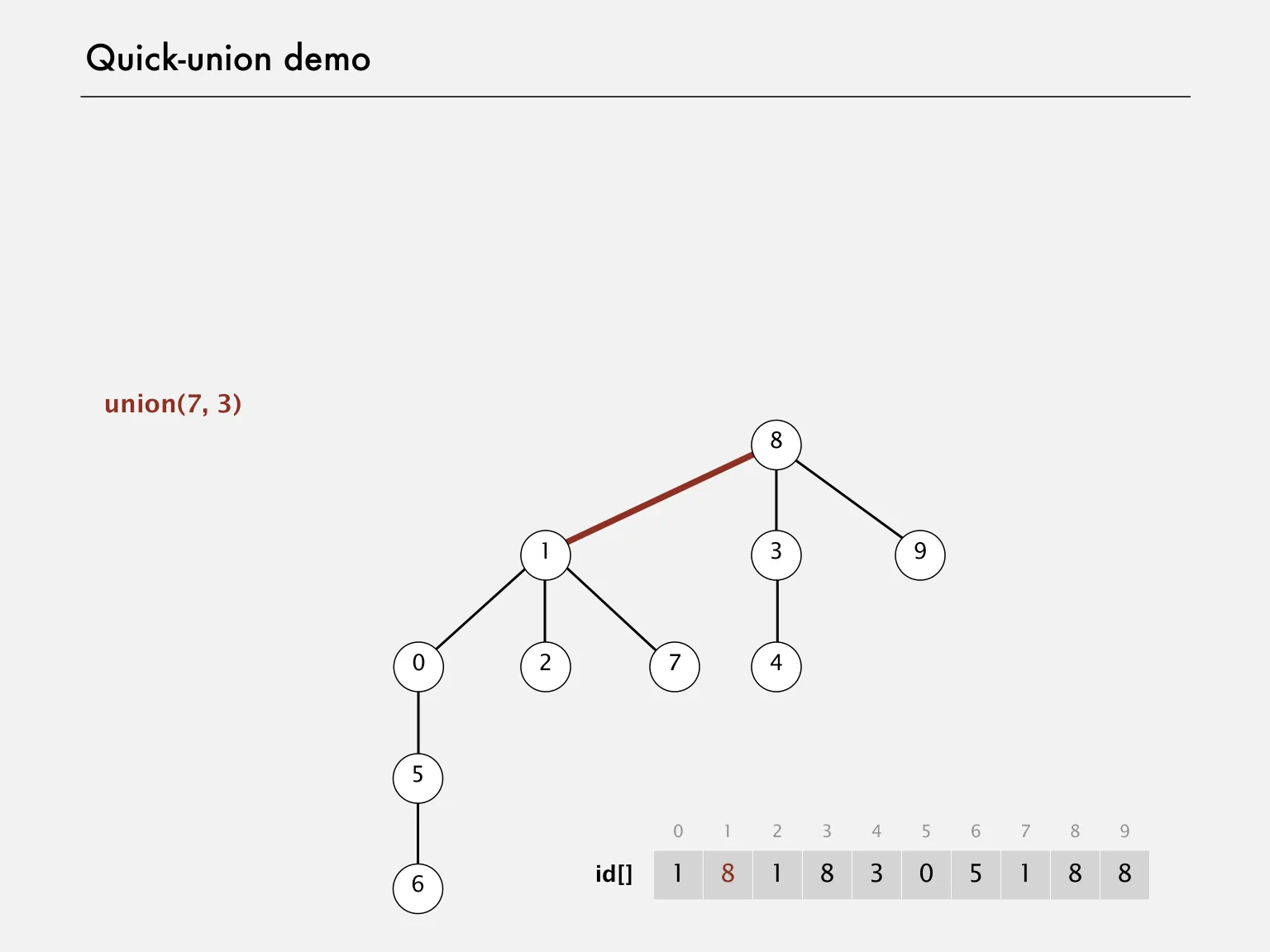
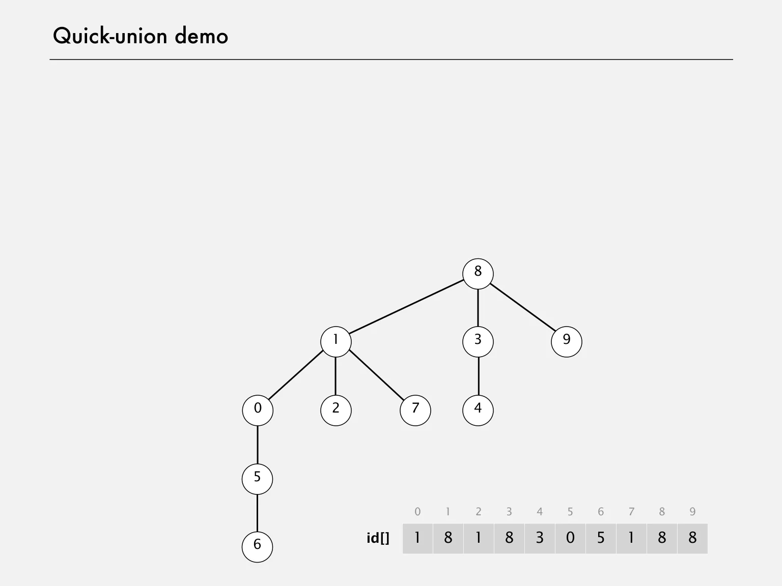
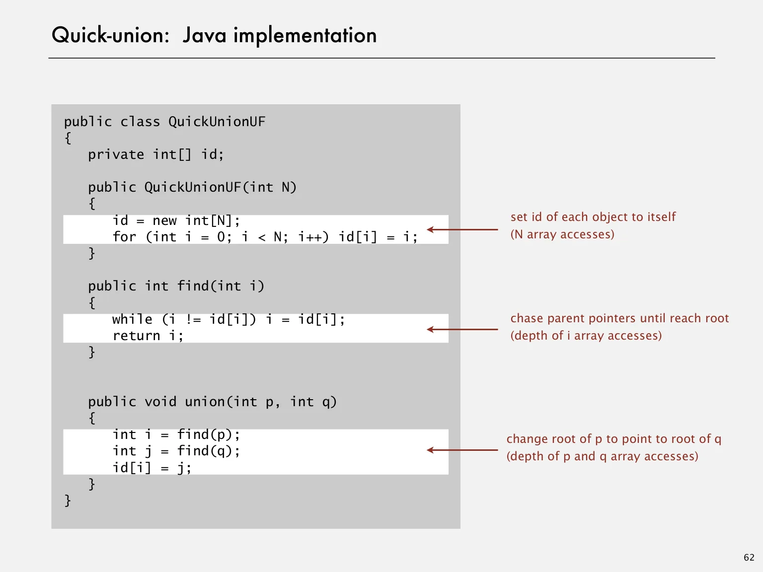
Interpret parent[p] as a link toward a root. A root points to itself. Find follows links until reaching a root; union makes one root point to the other. The structure represents a forest of trees.
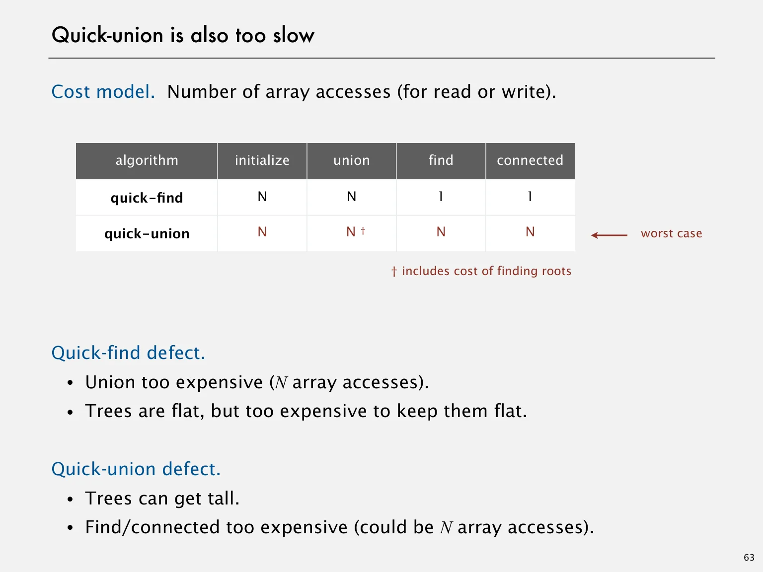
Unweighted linking can create a chain of length n−1. Both find and union can take Θ(n) in the worst case. The fact that union changes only one pointer does not make its root searches constant time.
Weighted union bounds the height
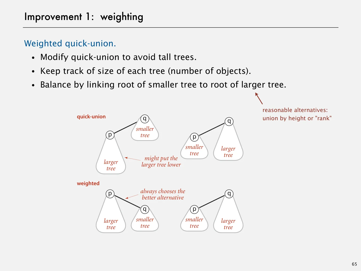
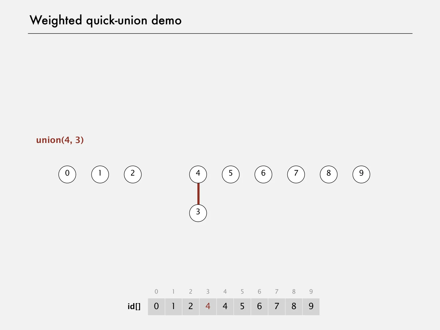
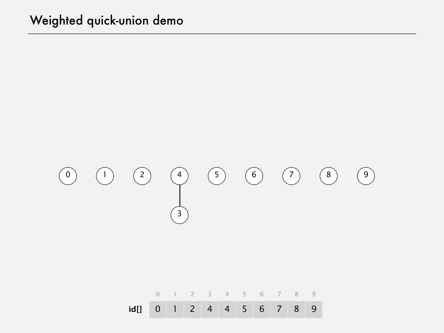
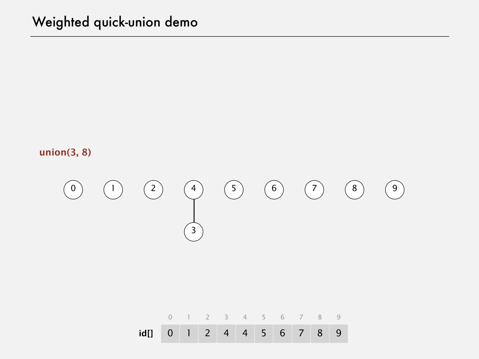
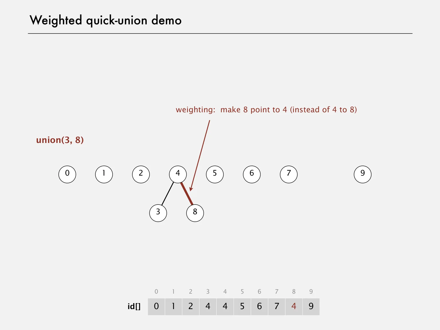
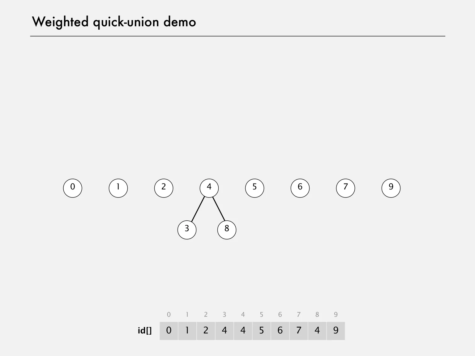
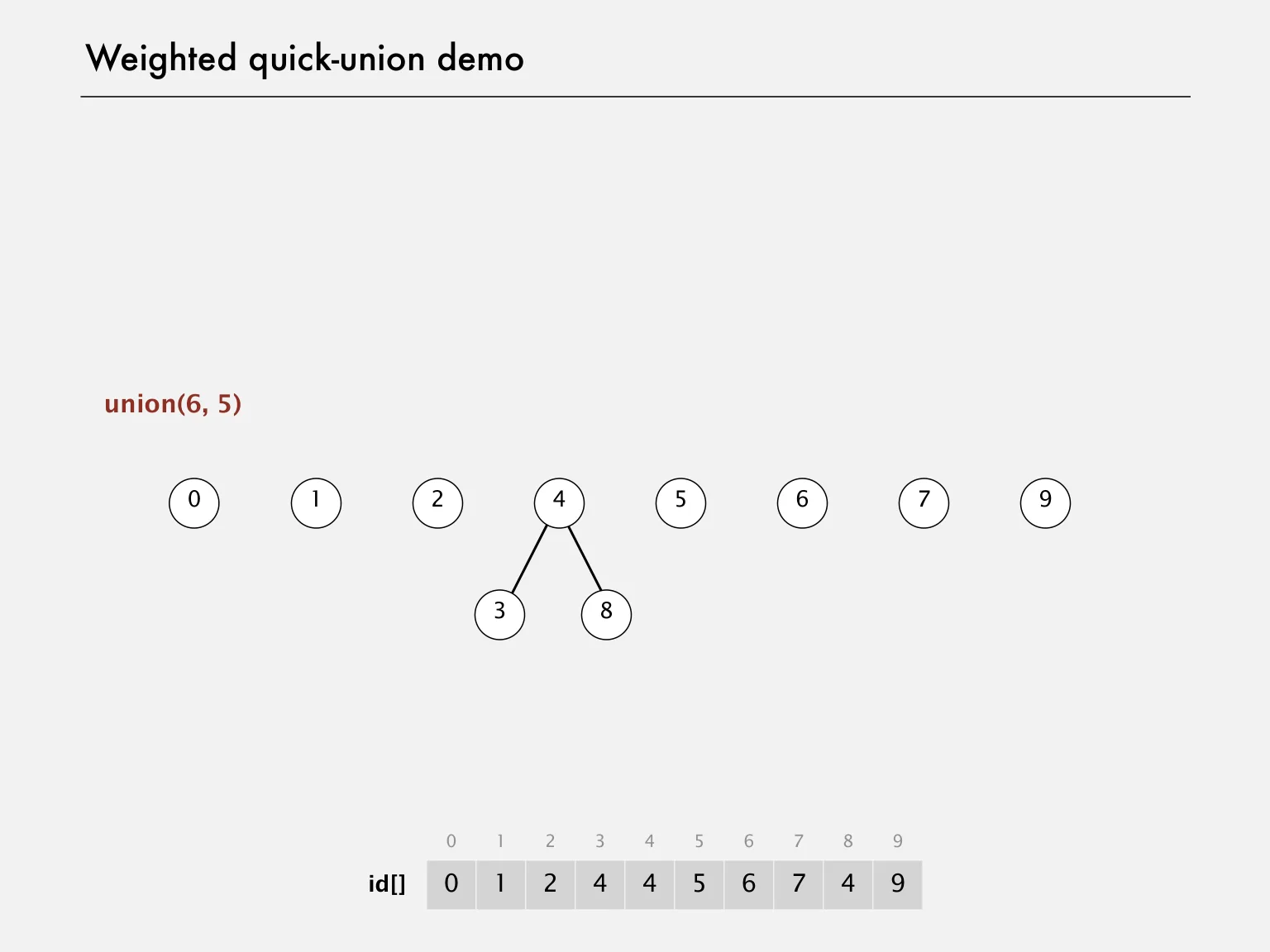
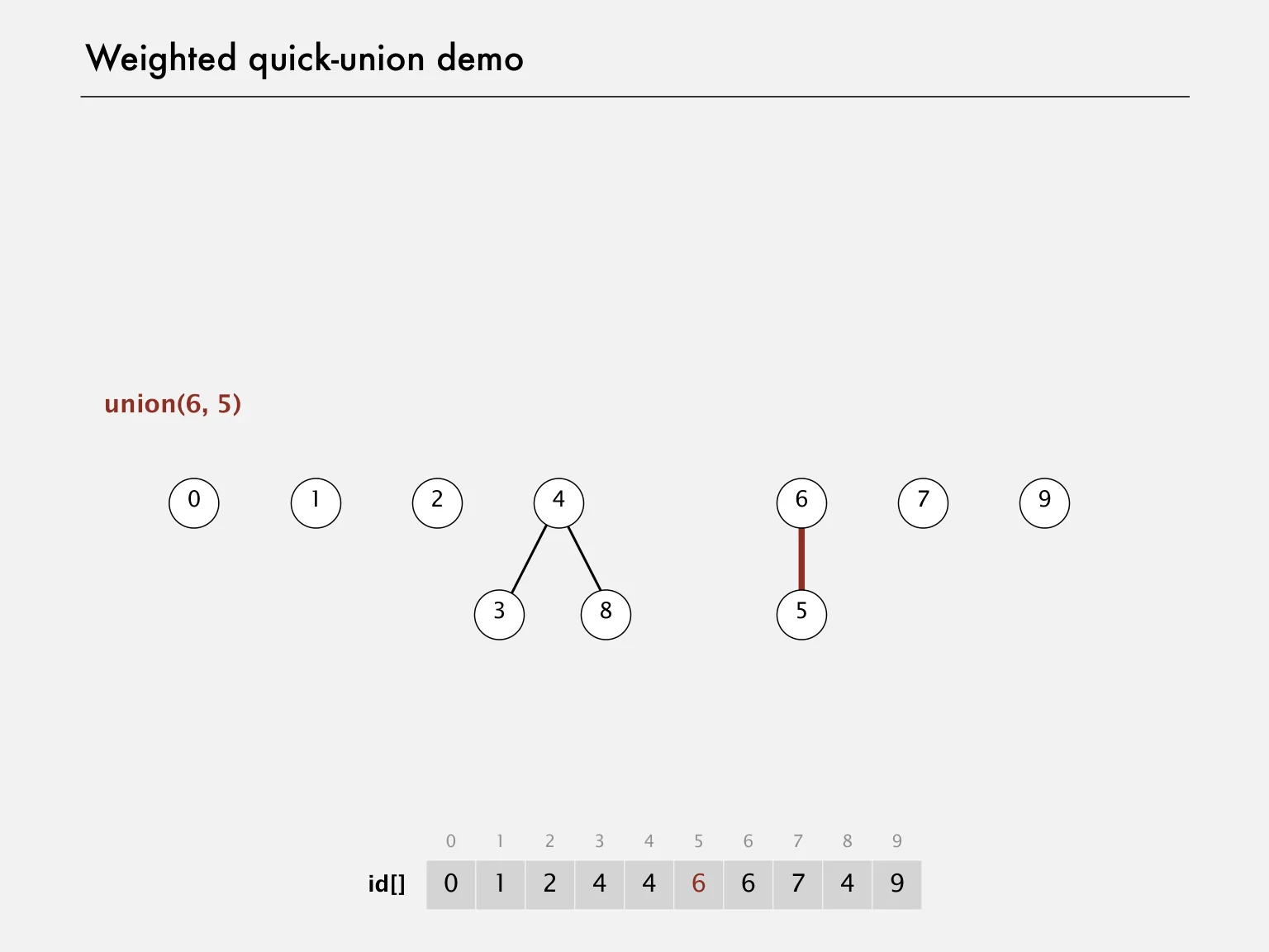
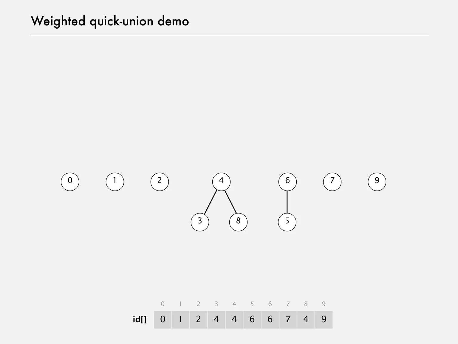
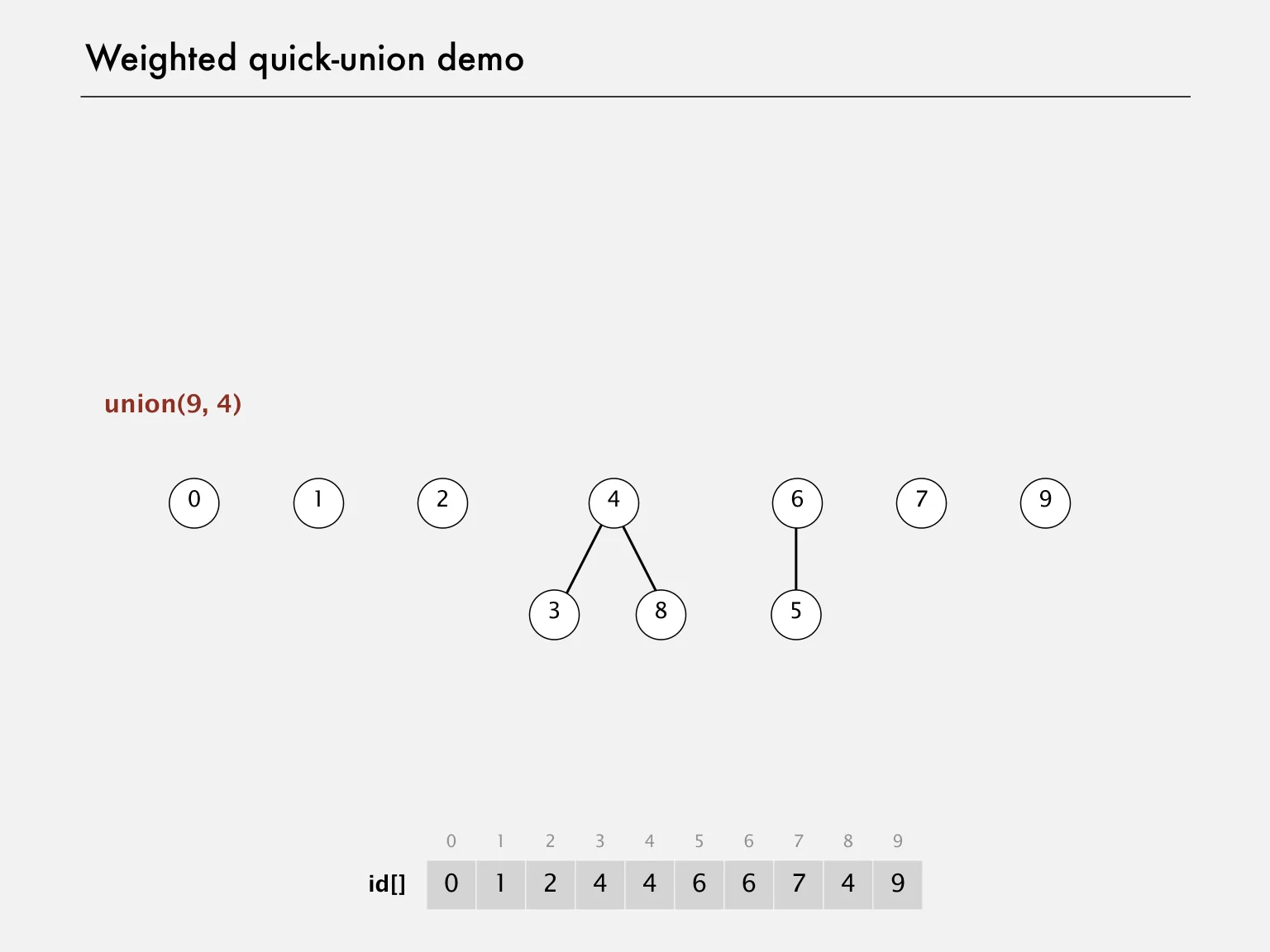
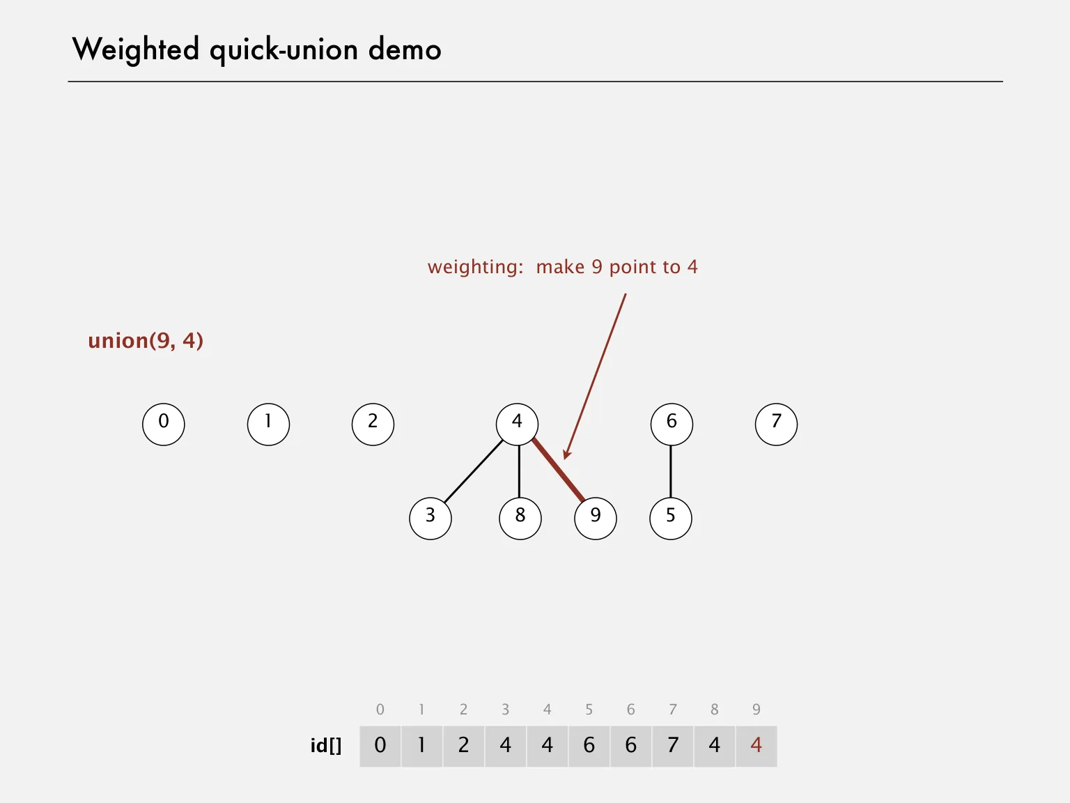
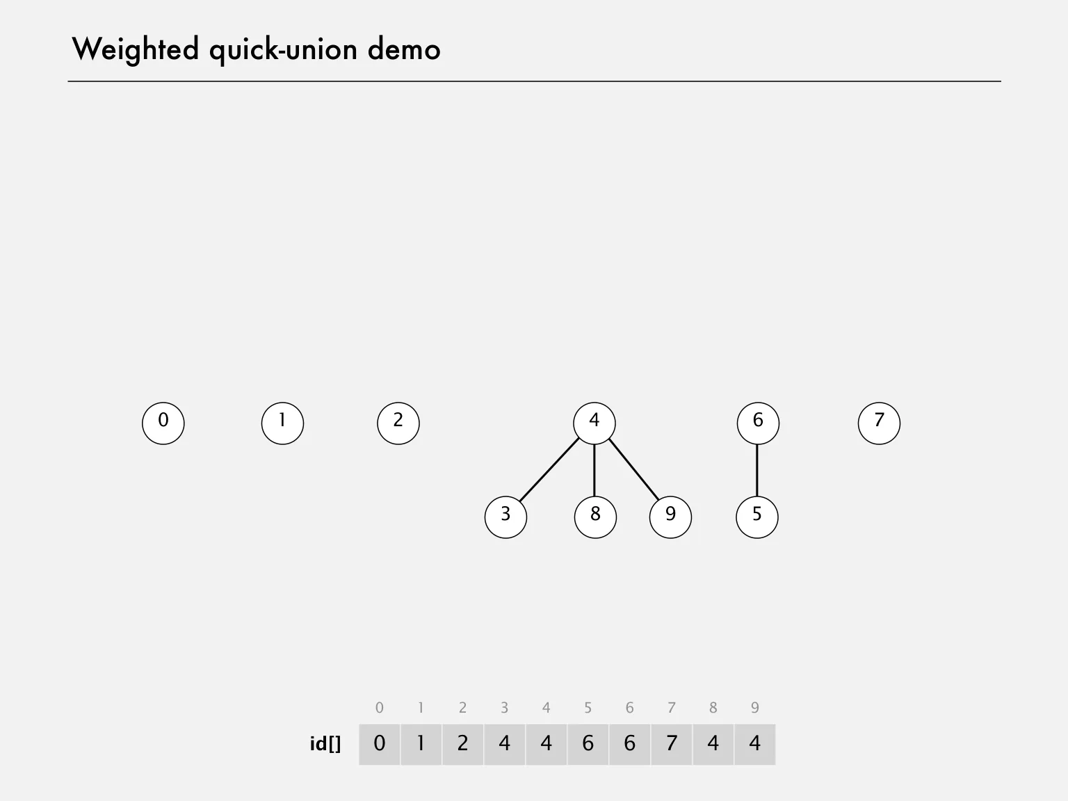
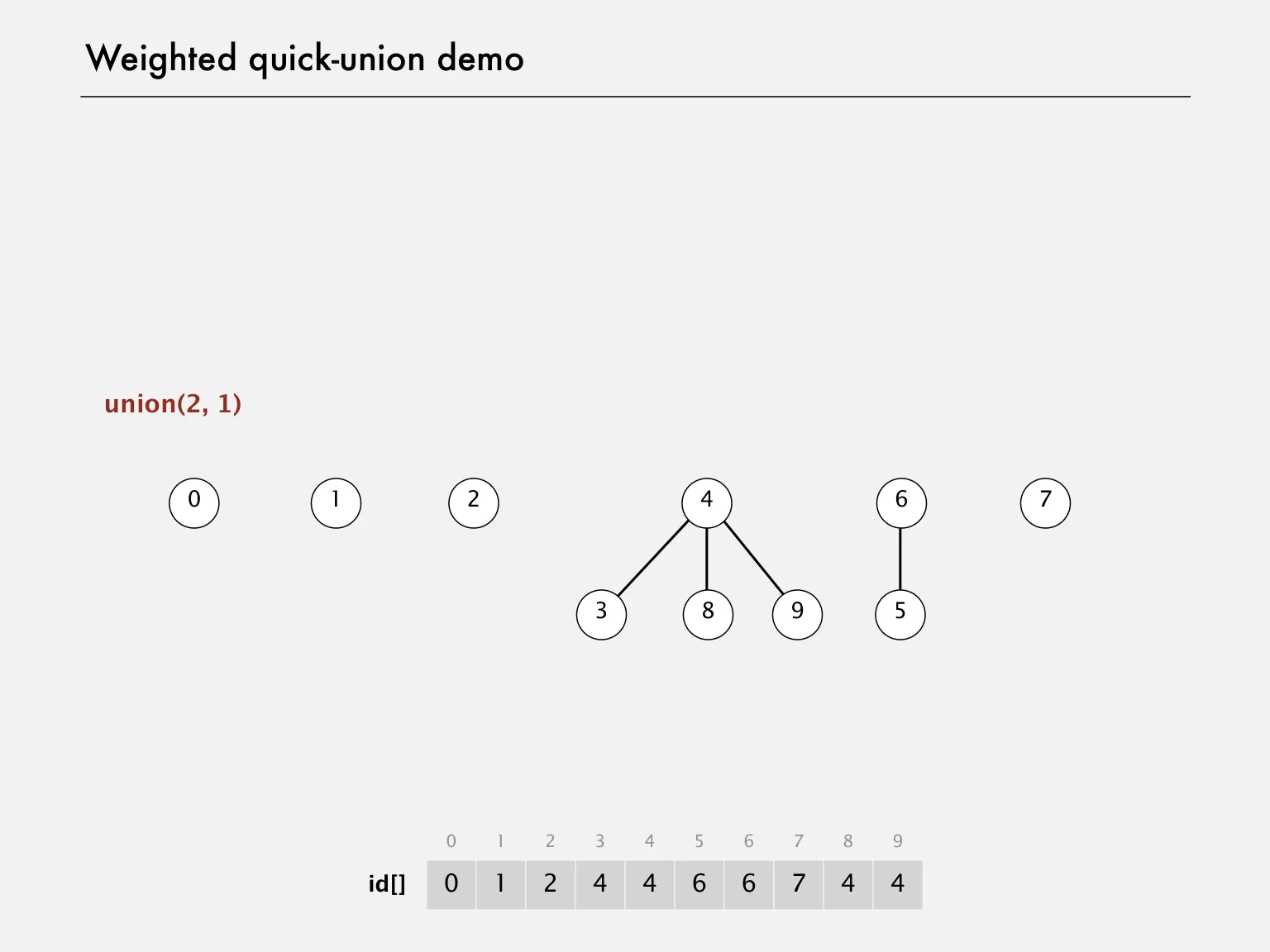
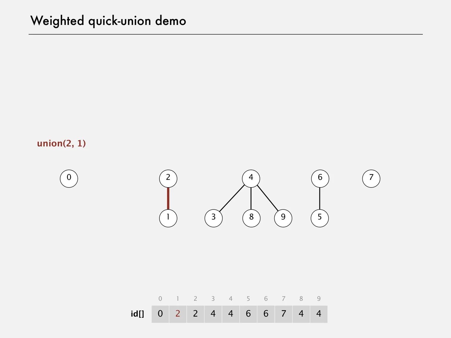
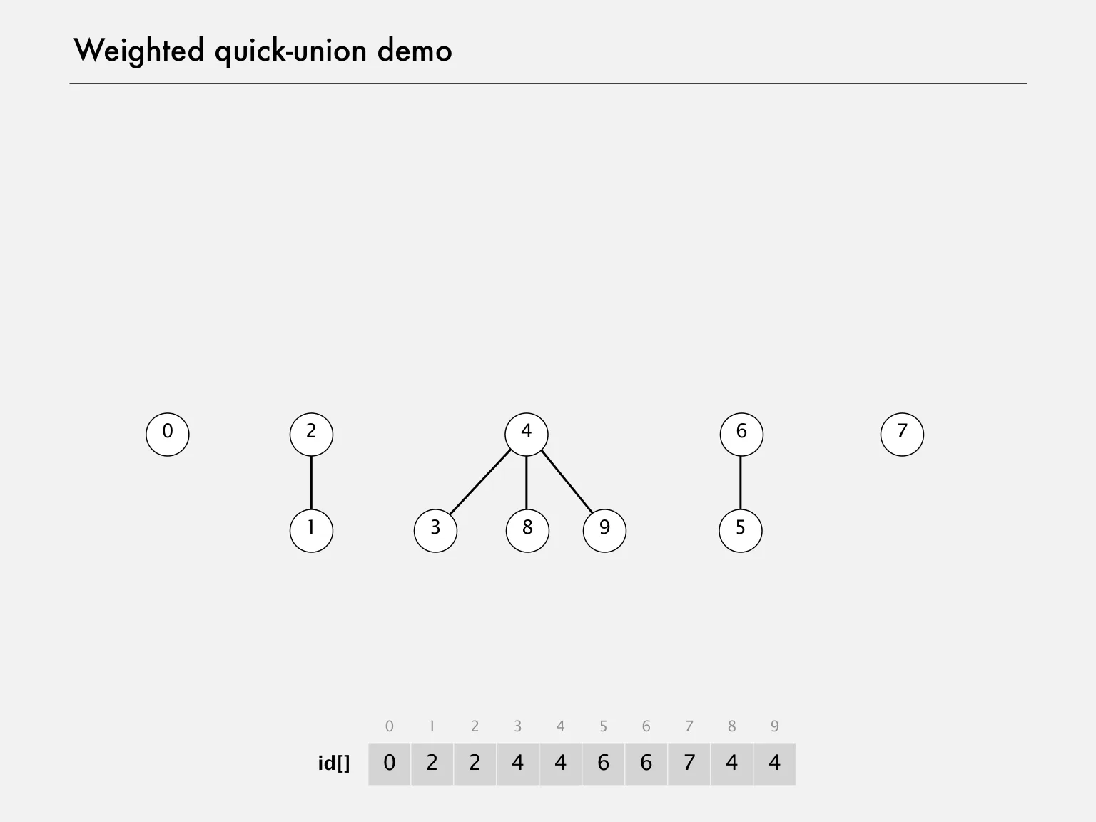
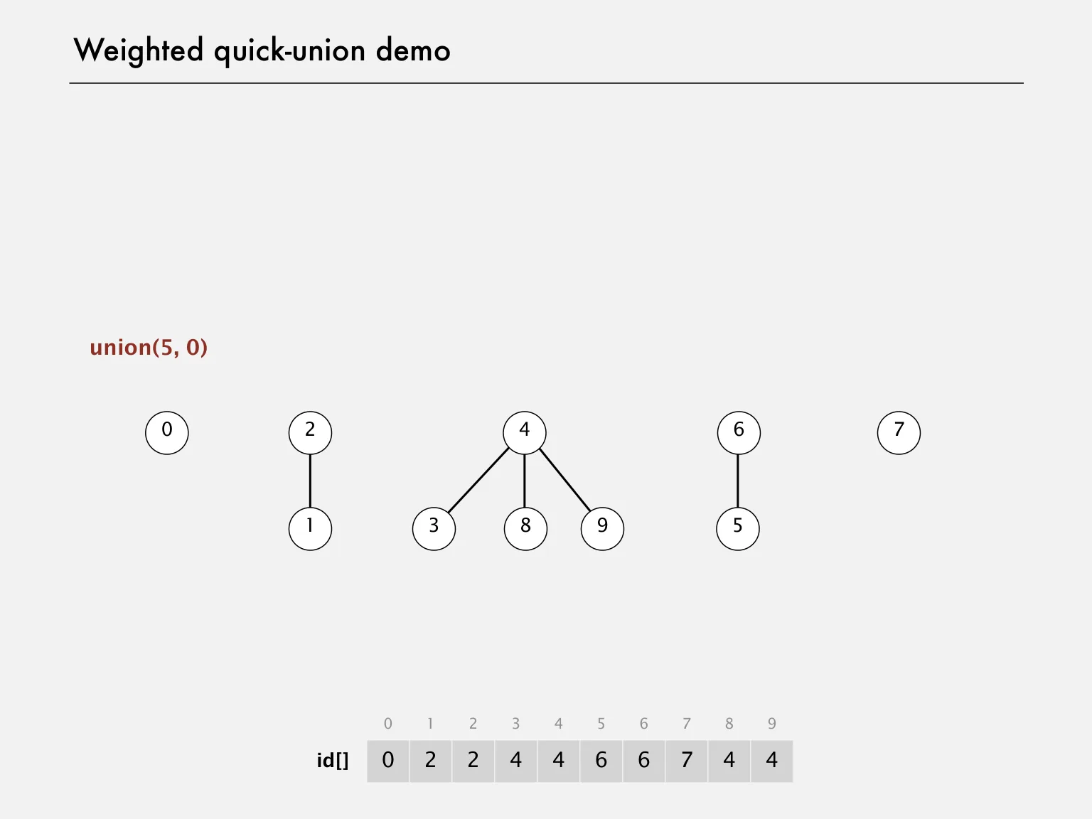
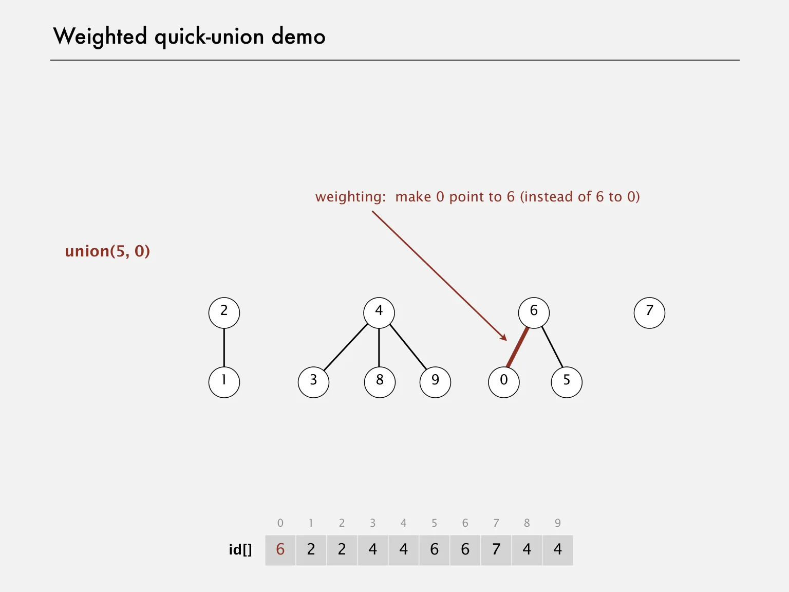
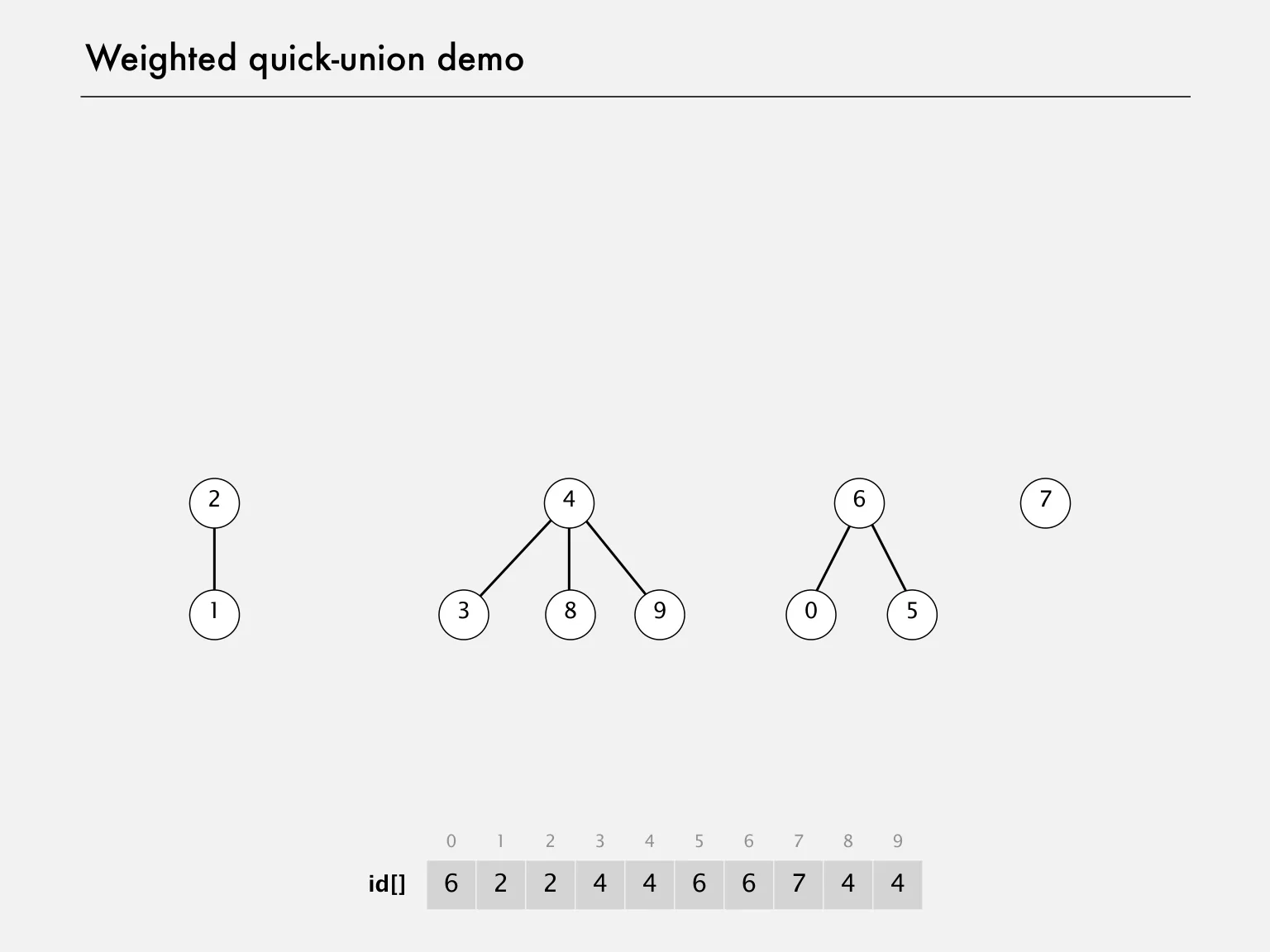
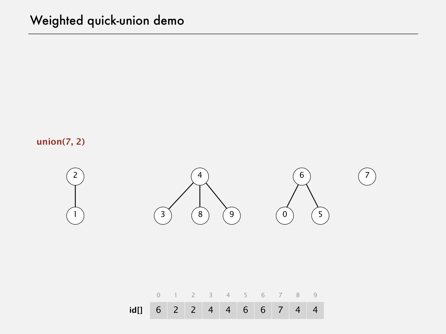
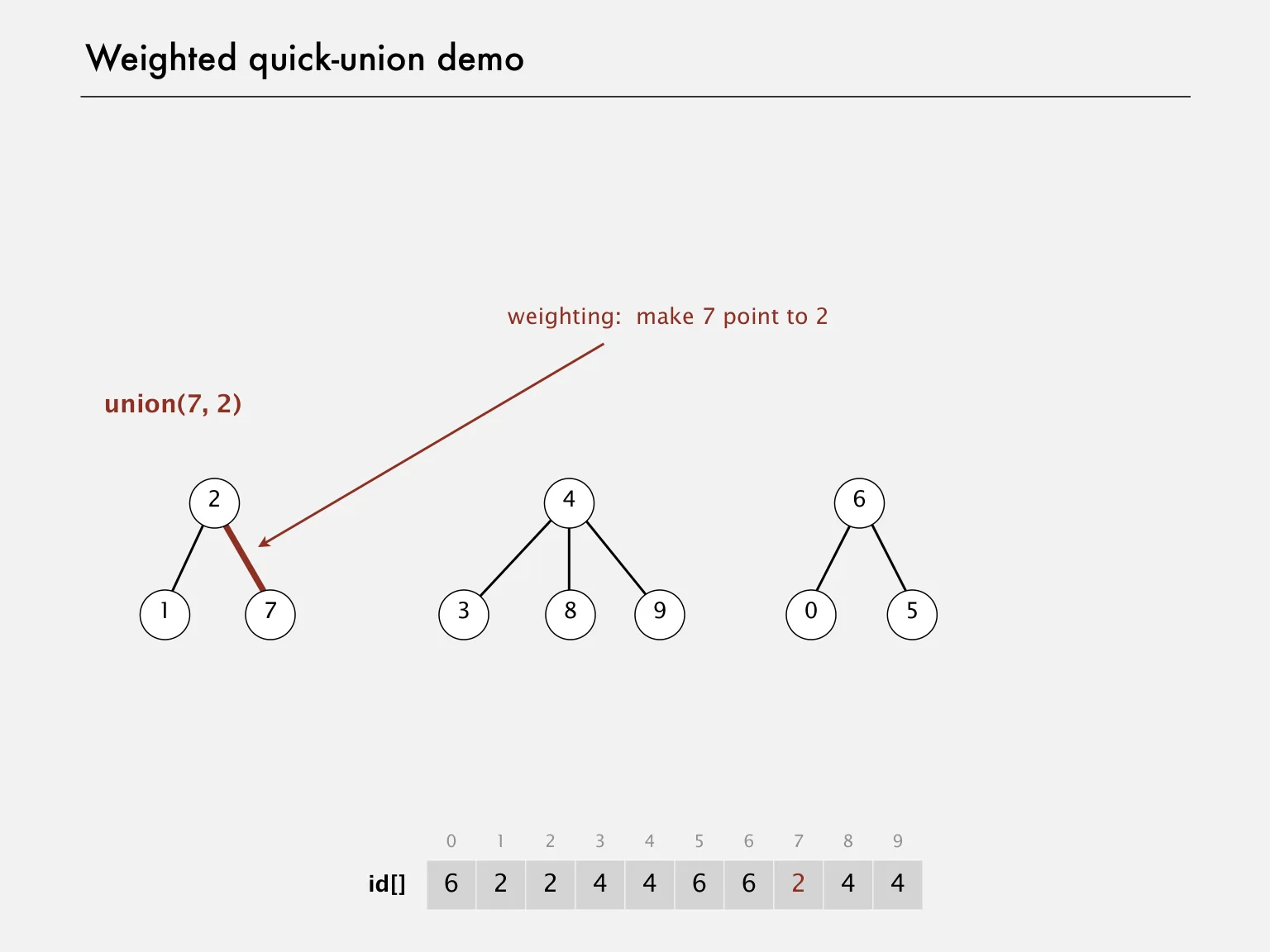
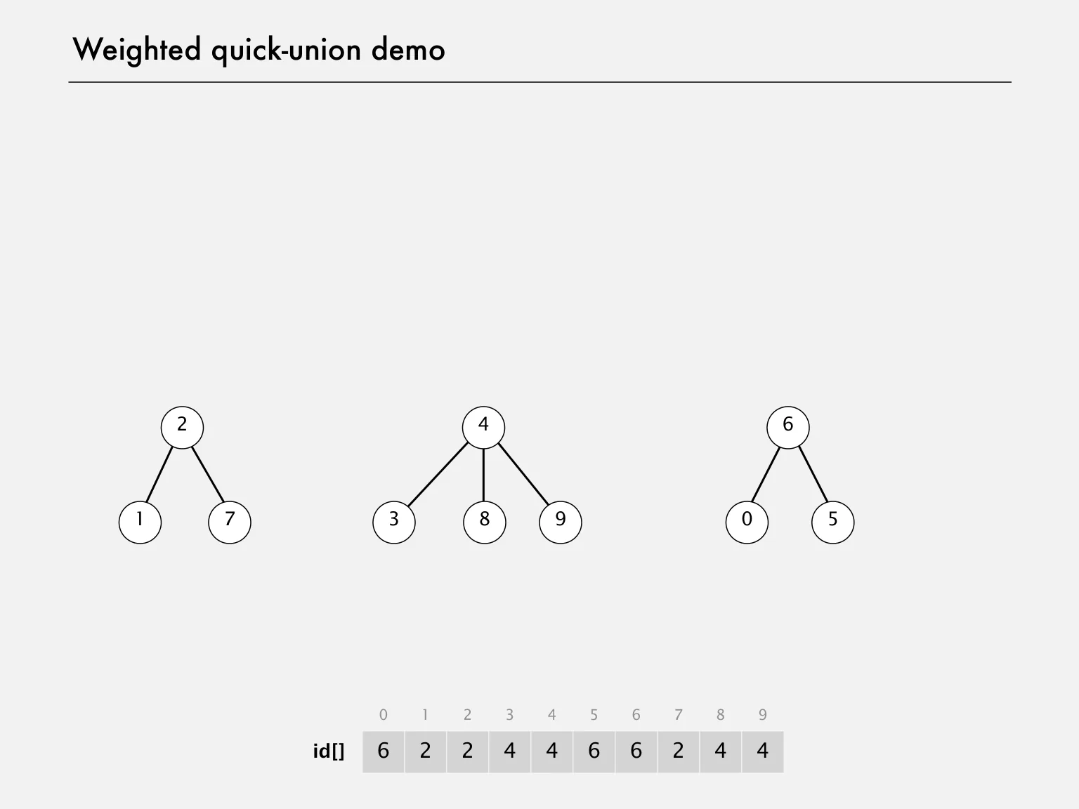
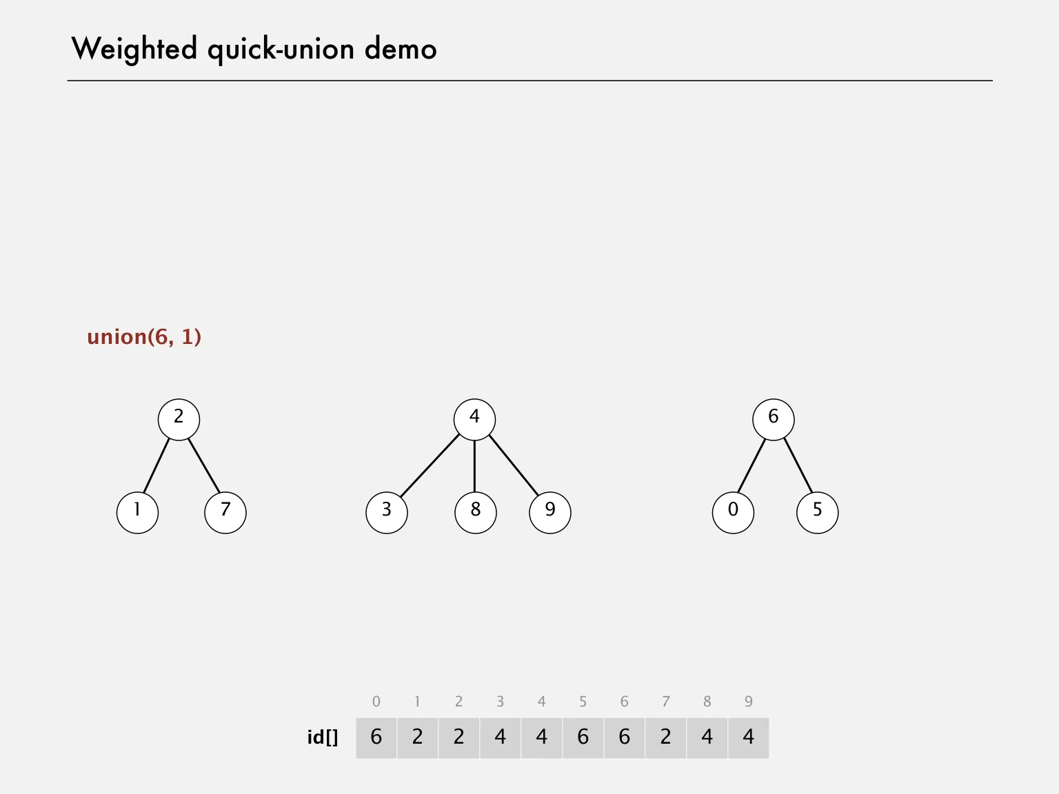
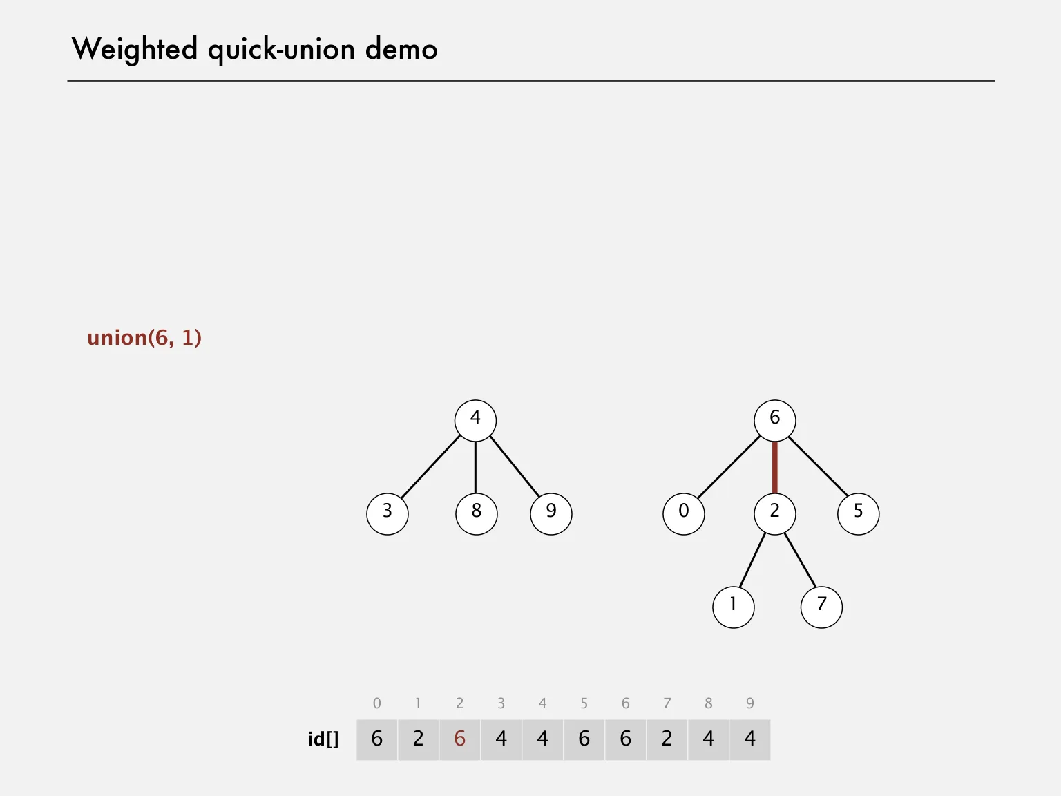
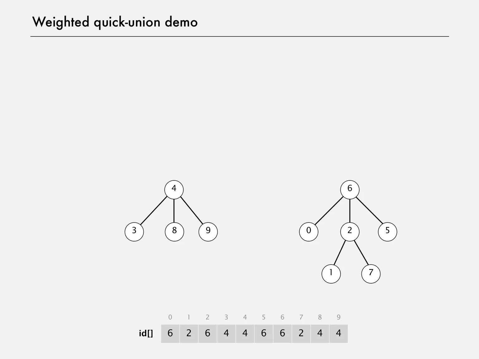
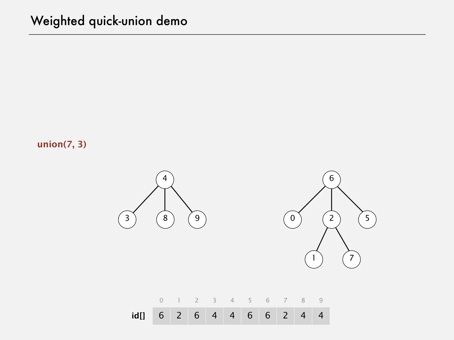
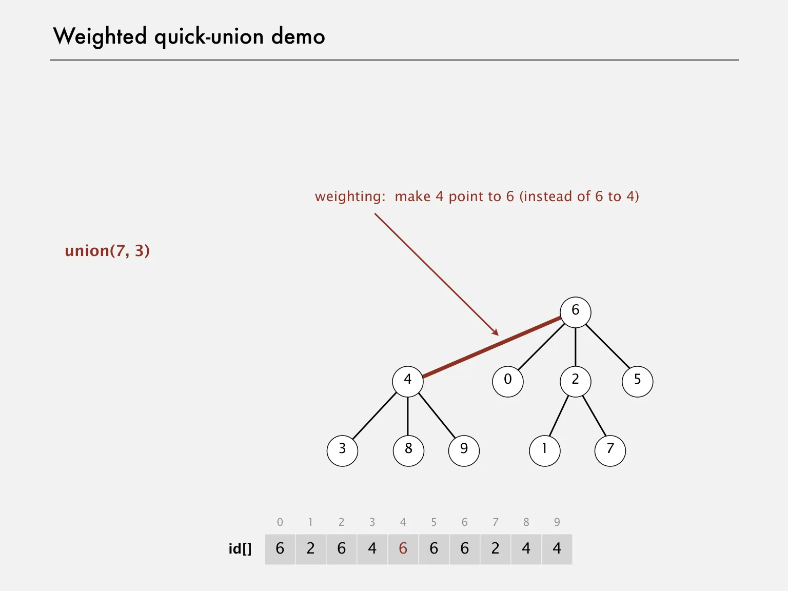
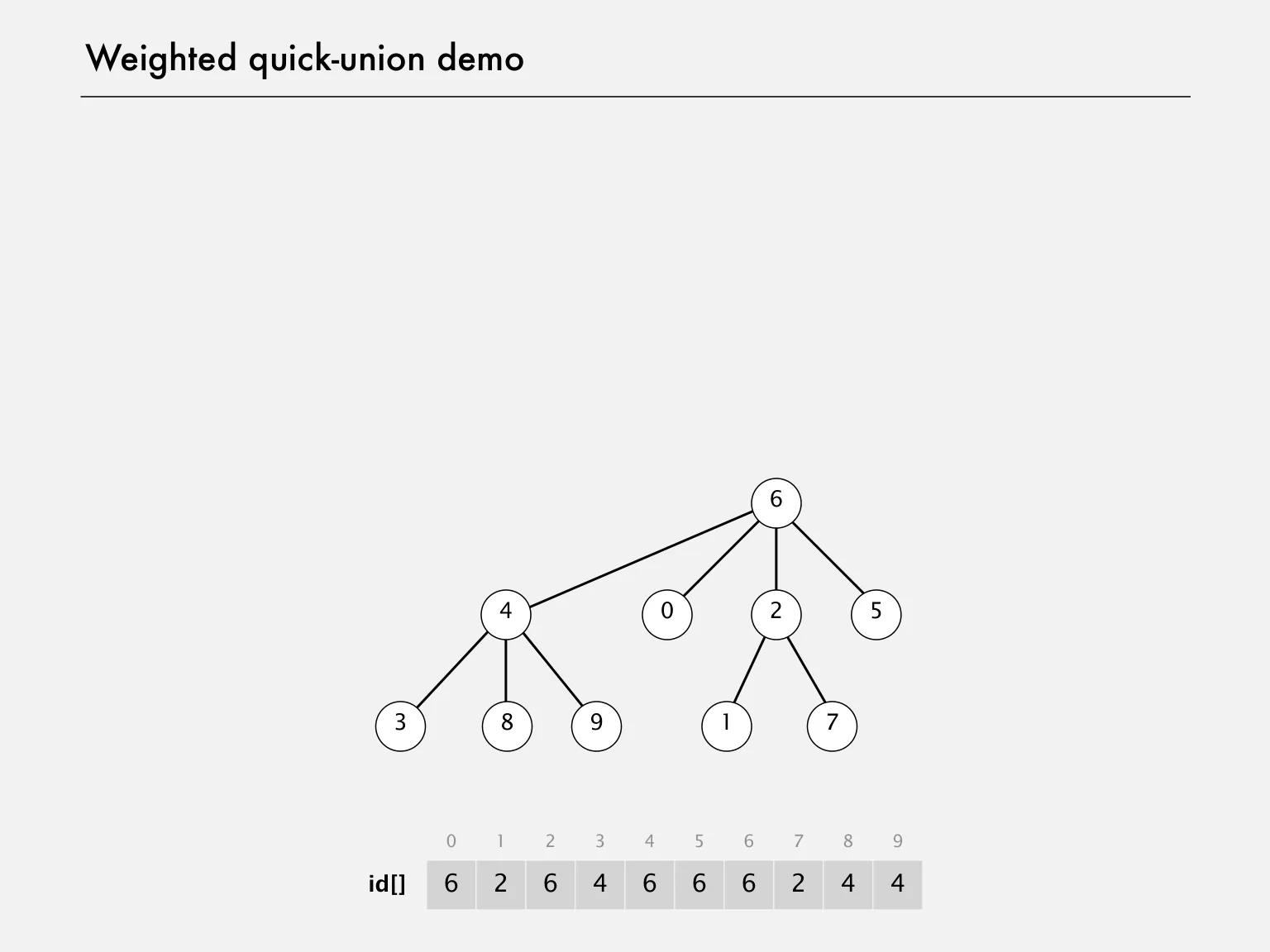
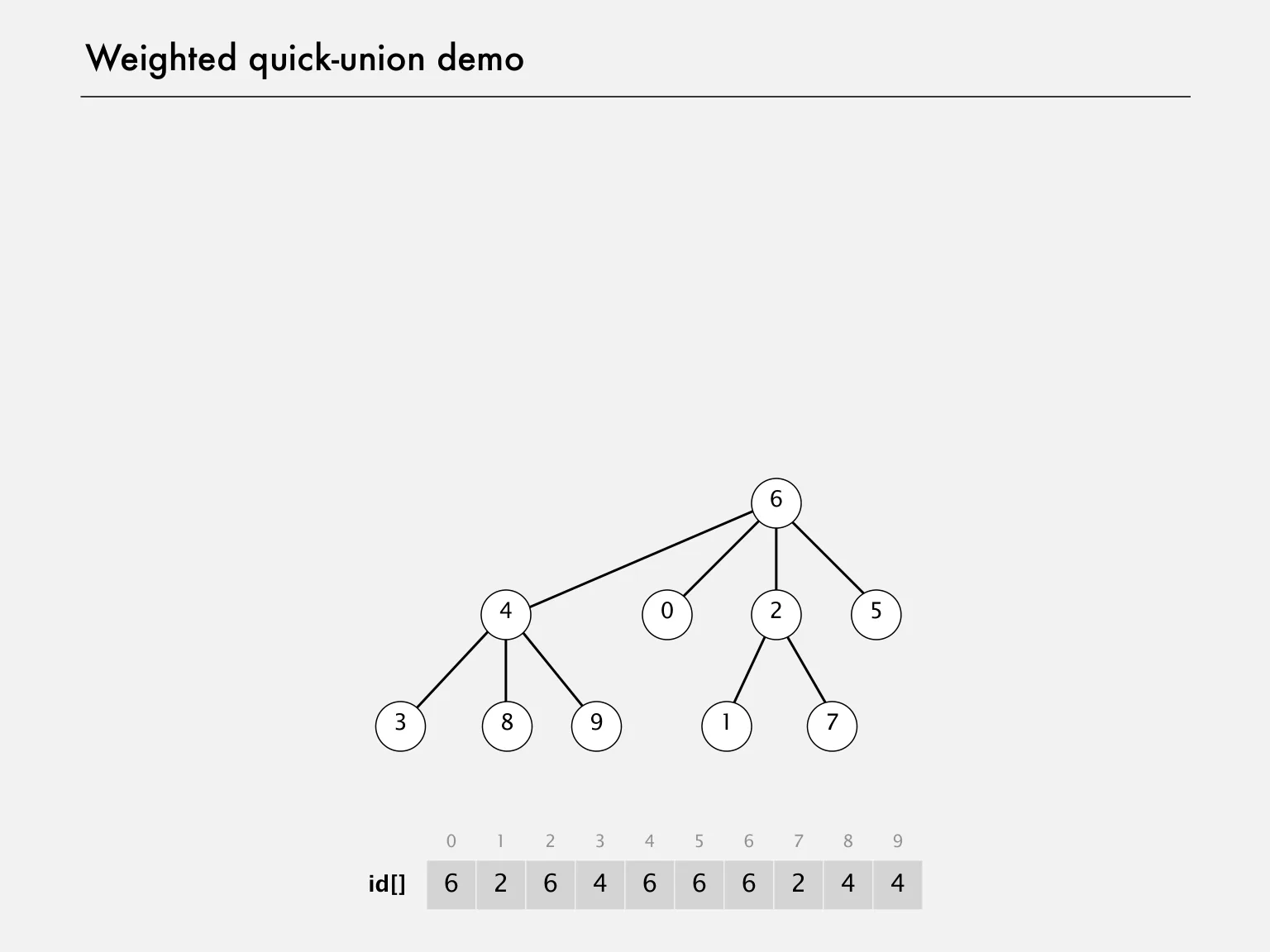
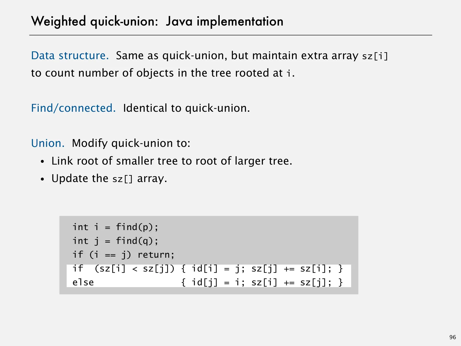
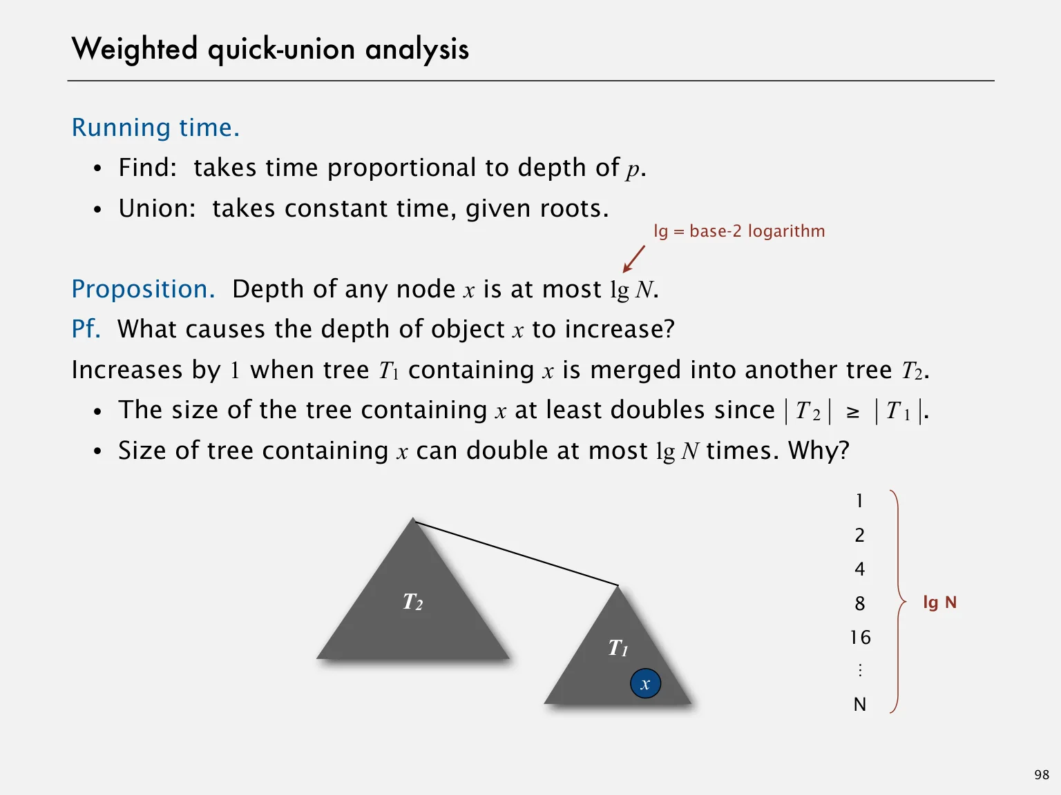
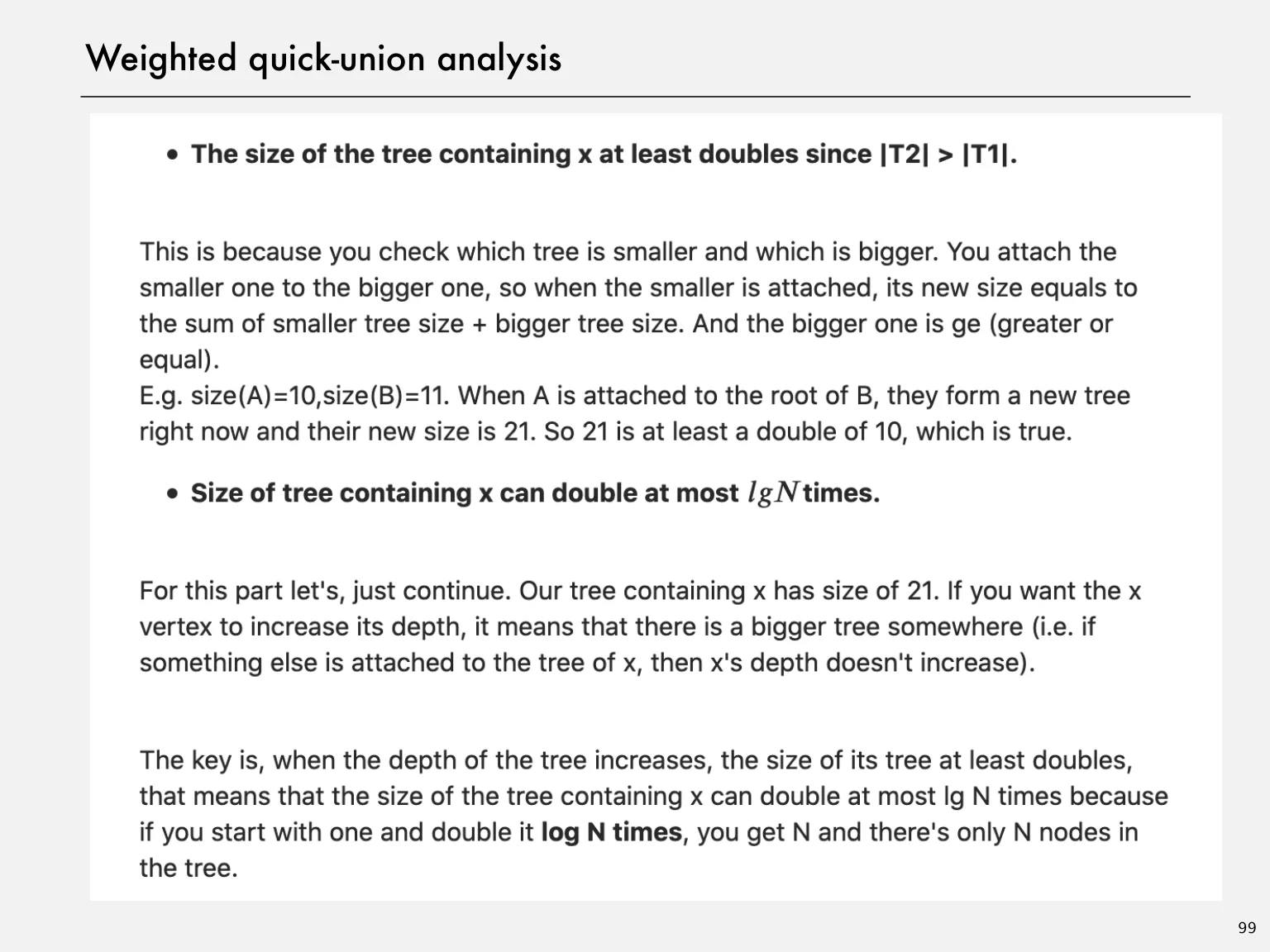
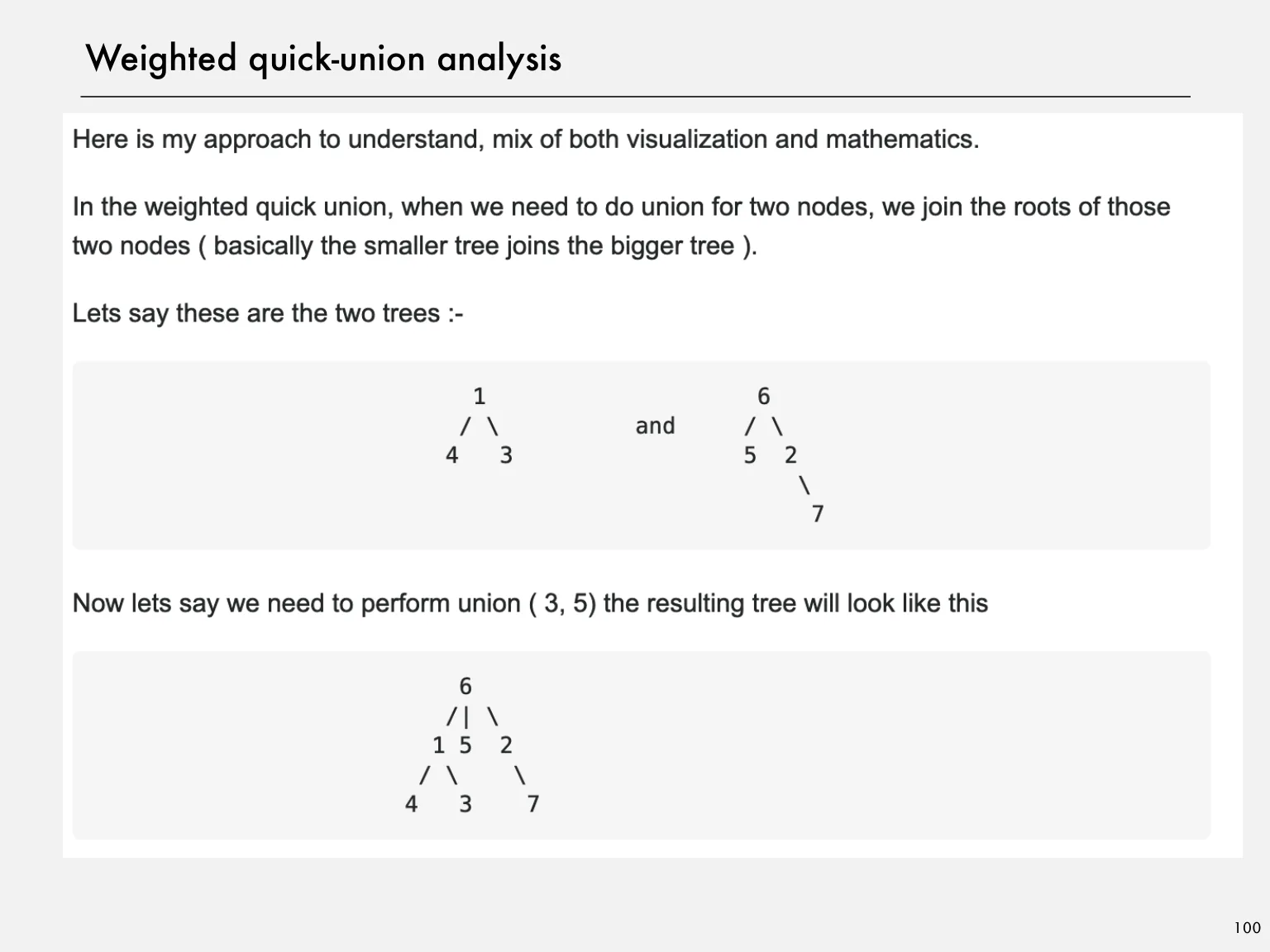
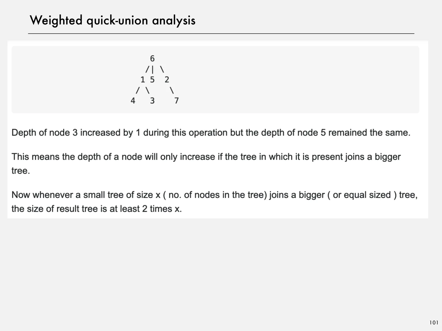
Keep the size of each tree at its root. Attach the smaller tree’s root beneath the larger tree’s root. The depth of a node increases only when its tree is attached to another tree at least as large, so the containing component at least doubles.
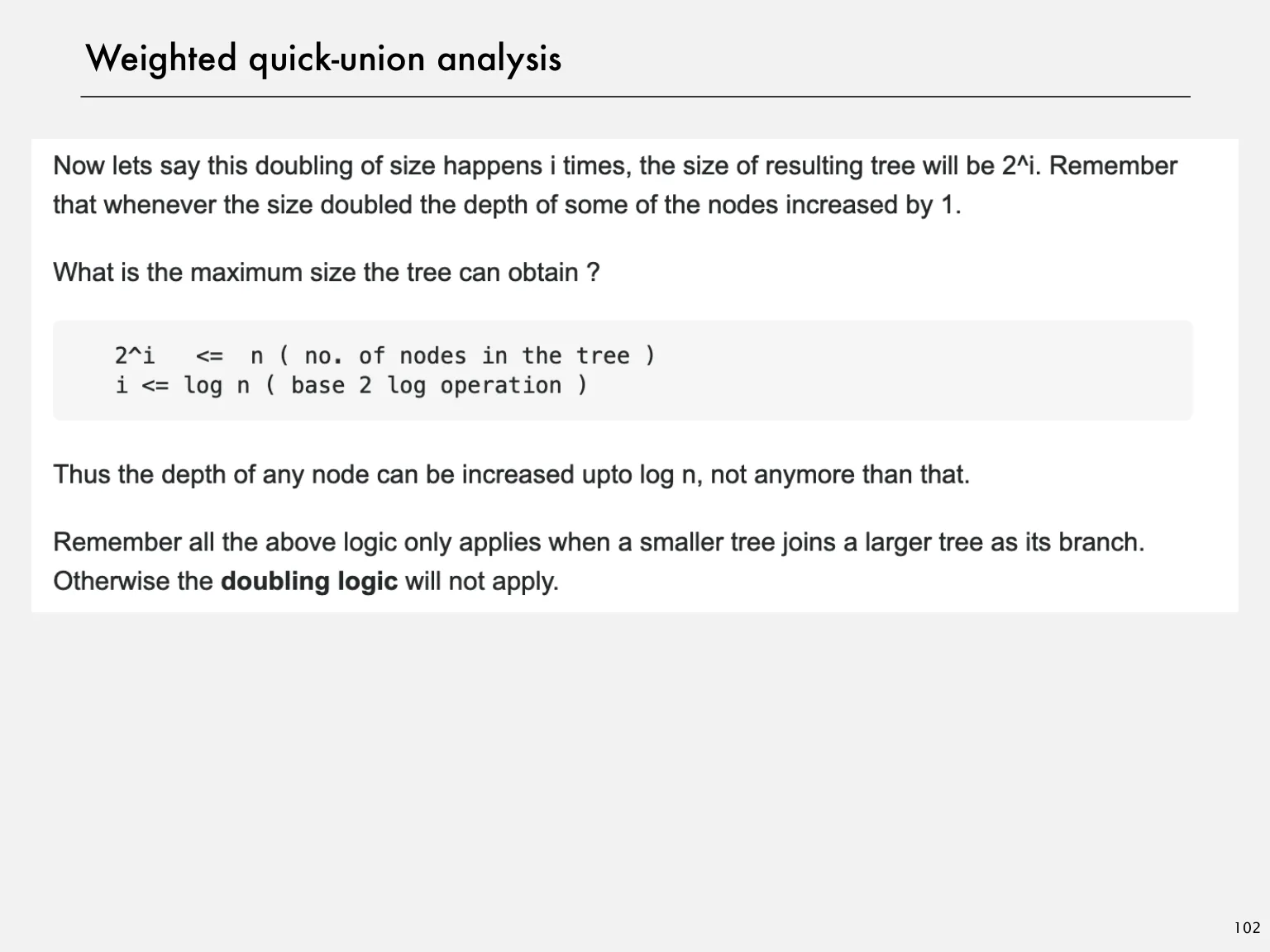
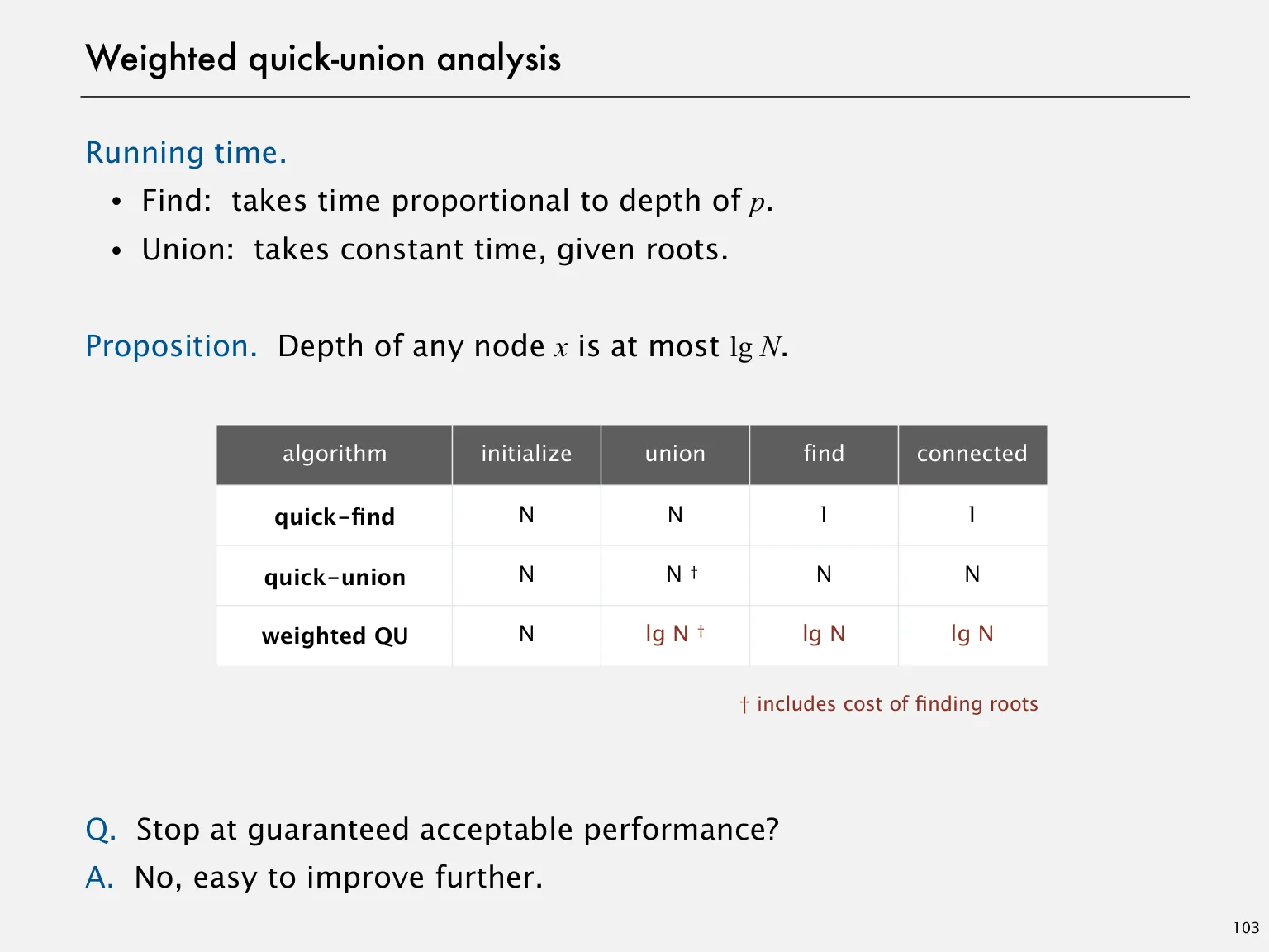
After a node’s depth increases k times, its tree contains at least 2ᵏ nodes. Since it contains at most n nodes, k ≤ log₂ n. Thus find and union have O(log n) worst-case time, using Θ(n) storage.
2k≤n⟹k≤⌊log2n⌋
Path compression and amortized cost
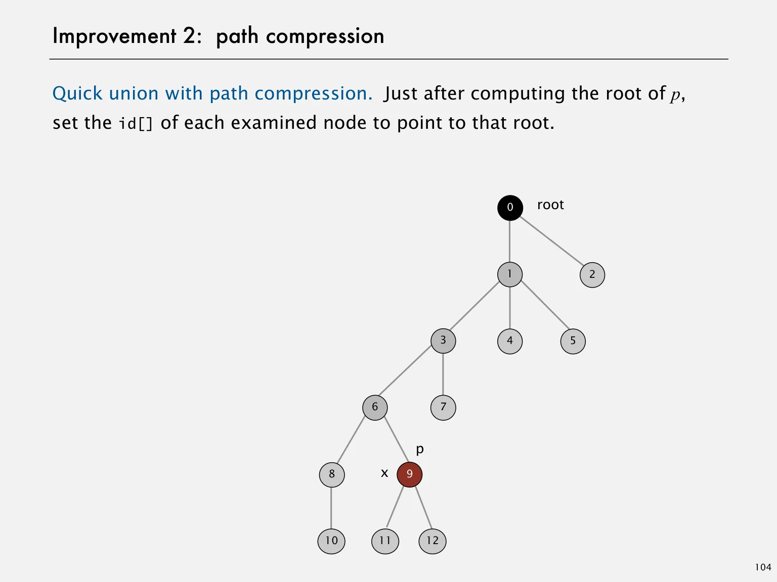
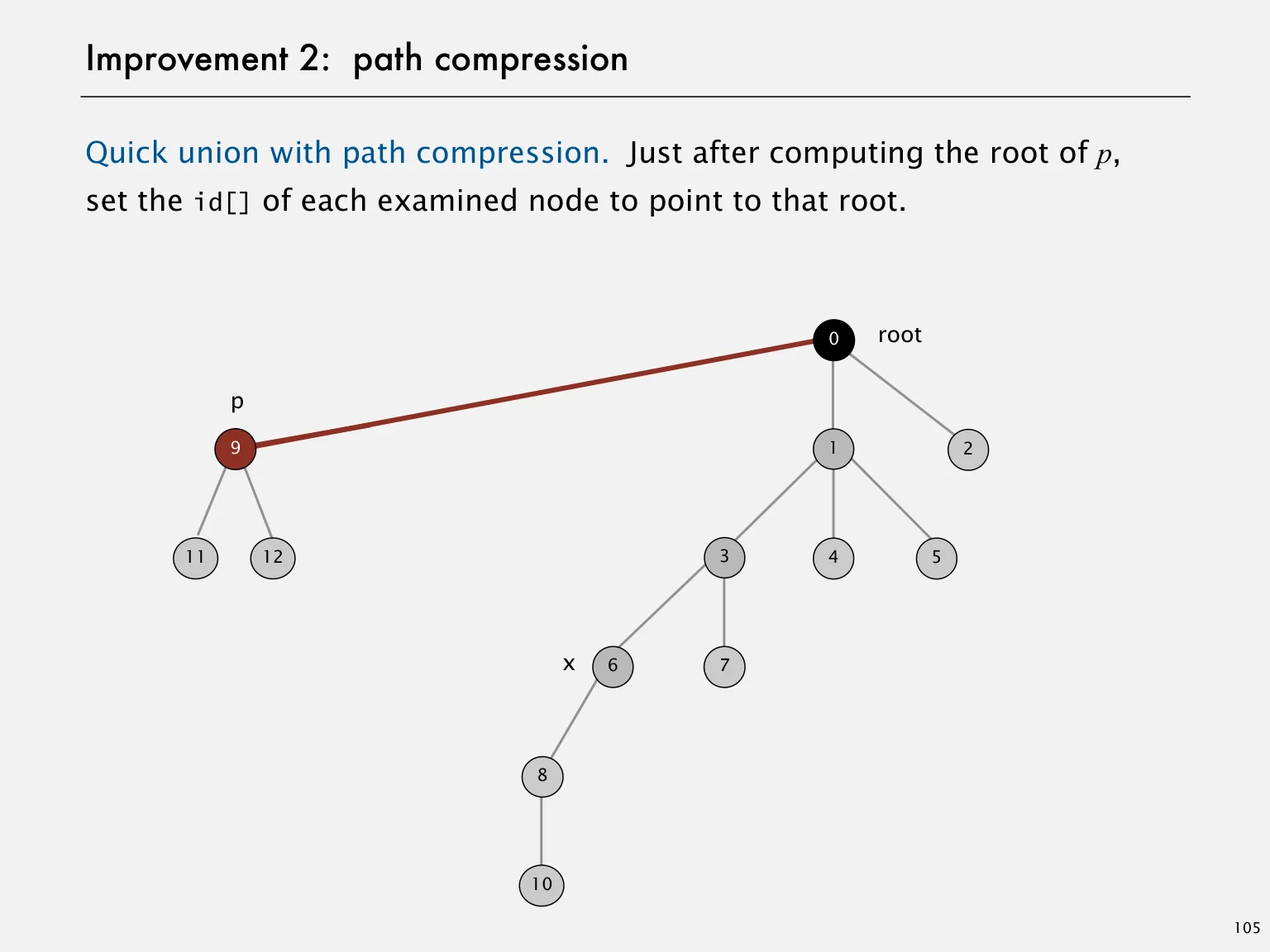
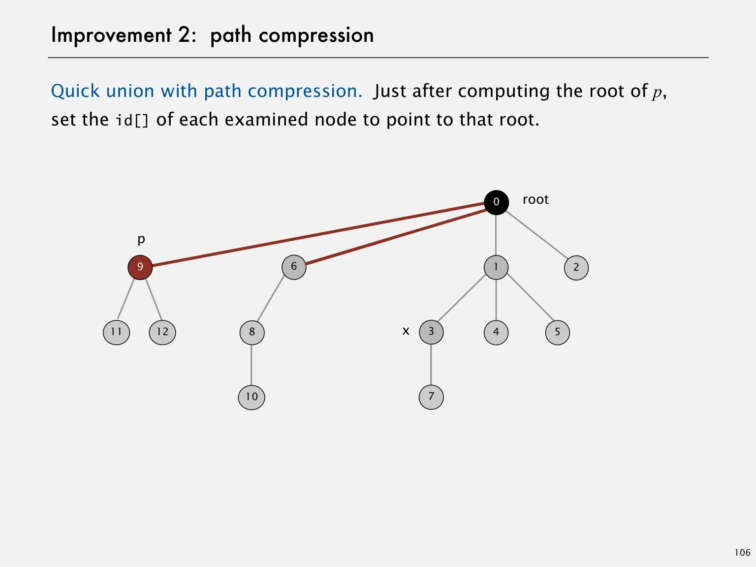
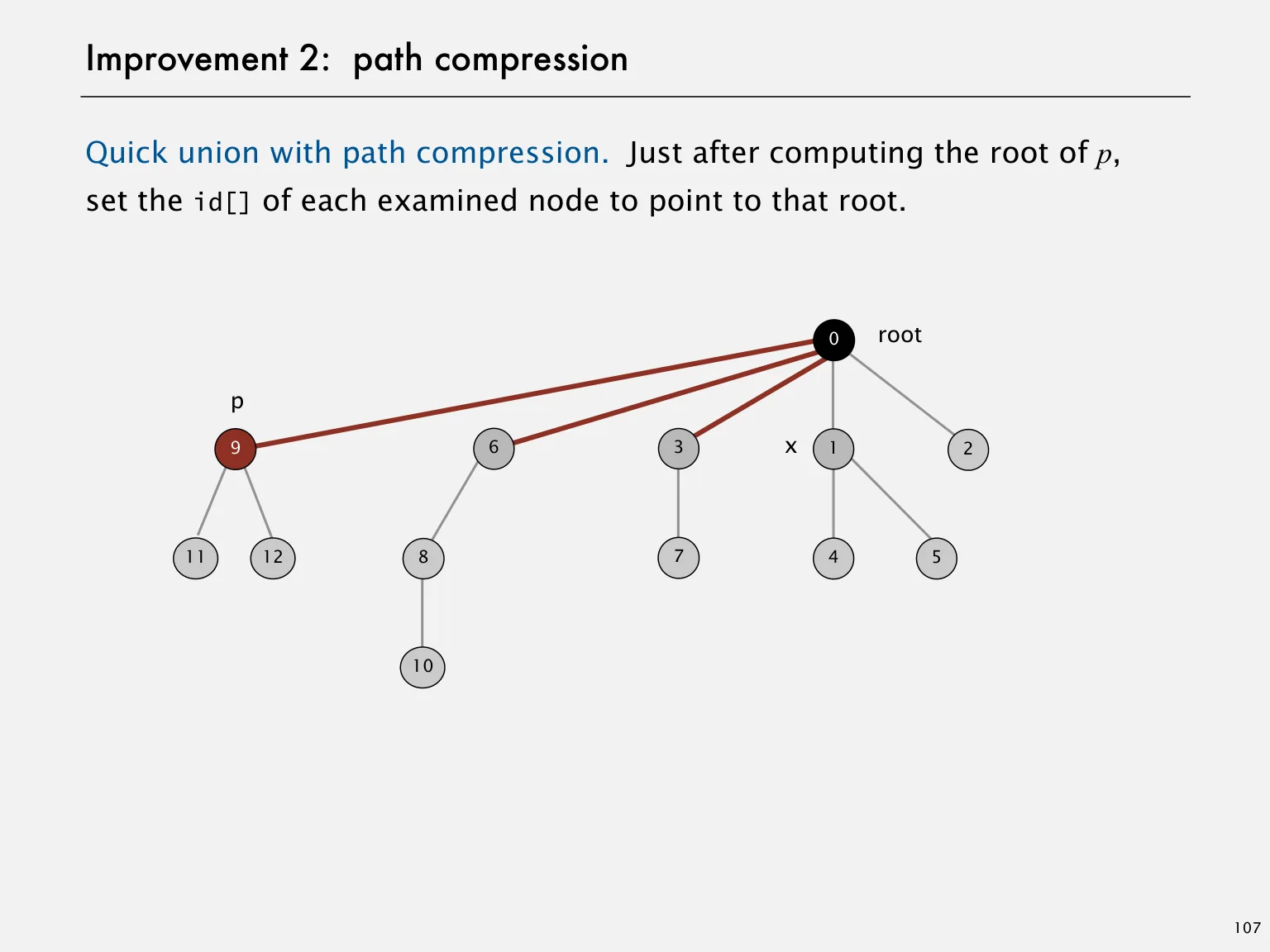
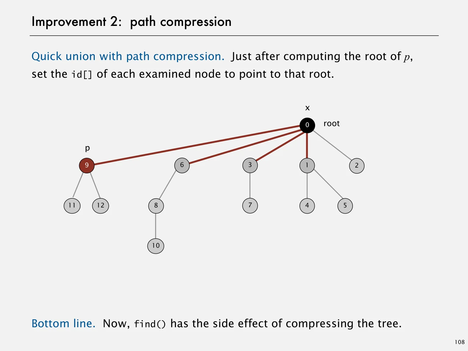
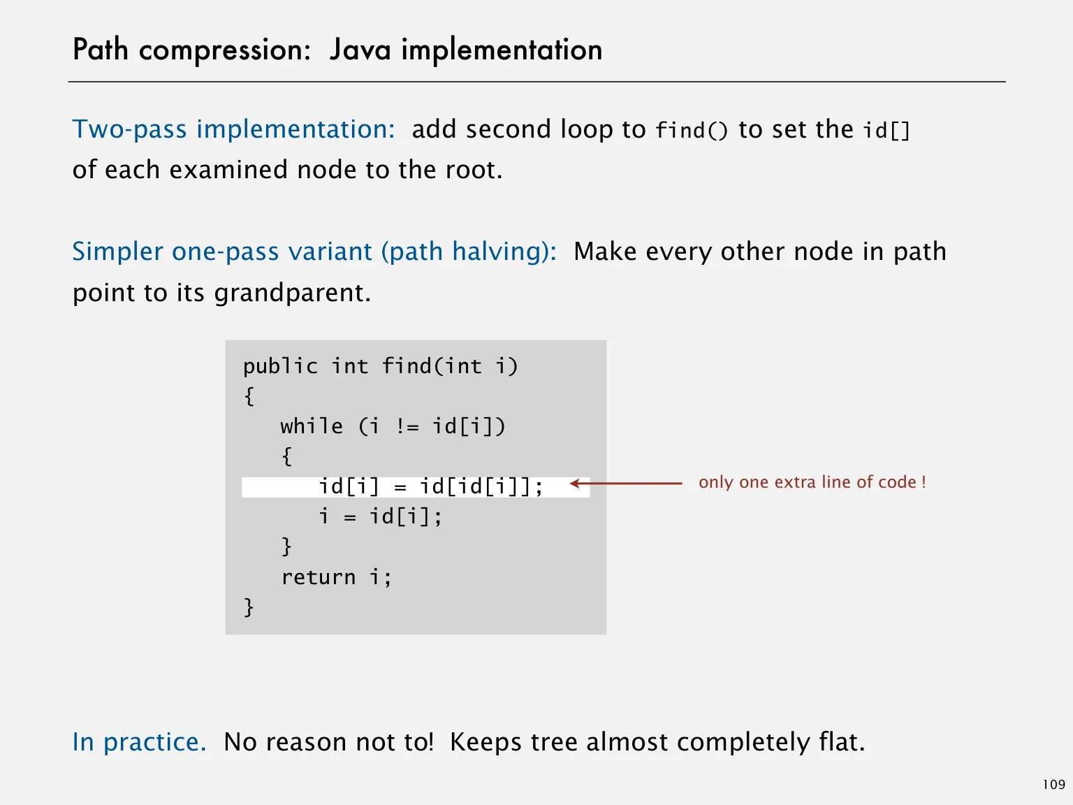
After locating a root, full path compression redirects the visited nodes directly to that root. Path halving is another variant that redirects links toward grandparents while searching. The supplied files contain different variants; do not silently treat them as identical implementations.
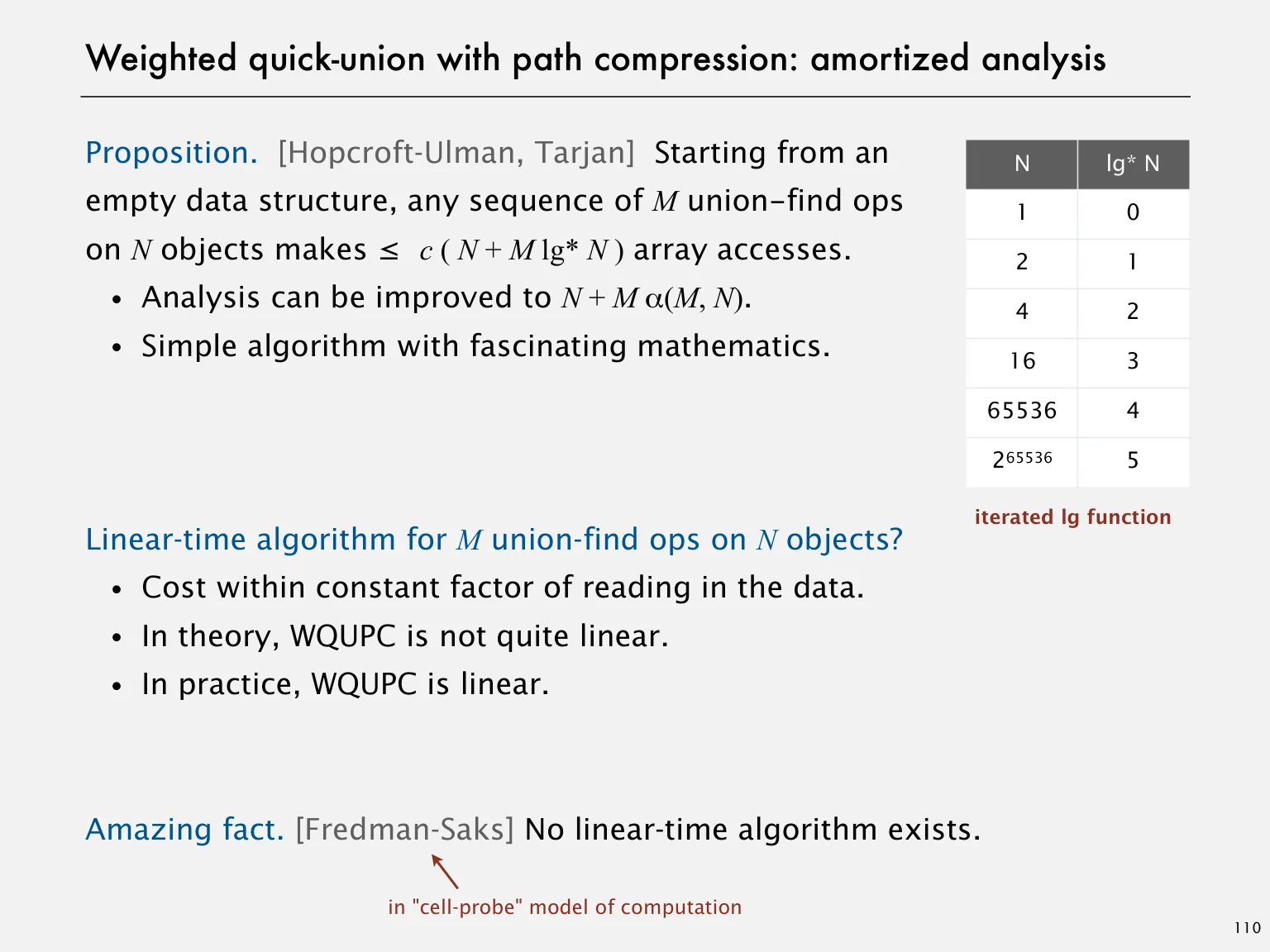
Weighting with compression gives extremely slow-growing amortized operation cost, conventionally expressed using the inverse Ackermann function α(n). This is a bound over a sequence, not a promise that every individual operation takes a fixed number of steps. Include Θ(n) initialization when measuring a complete run.
Application: percolation
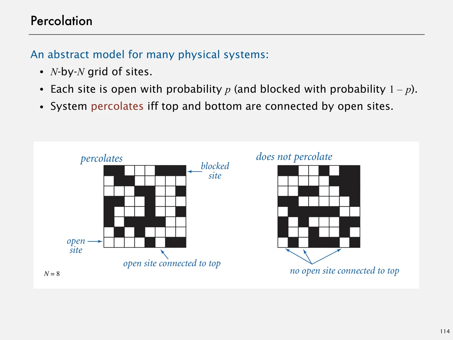
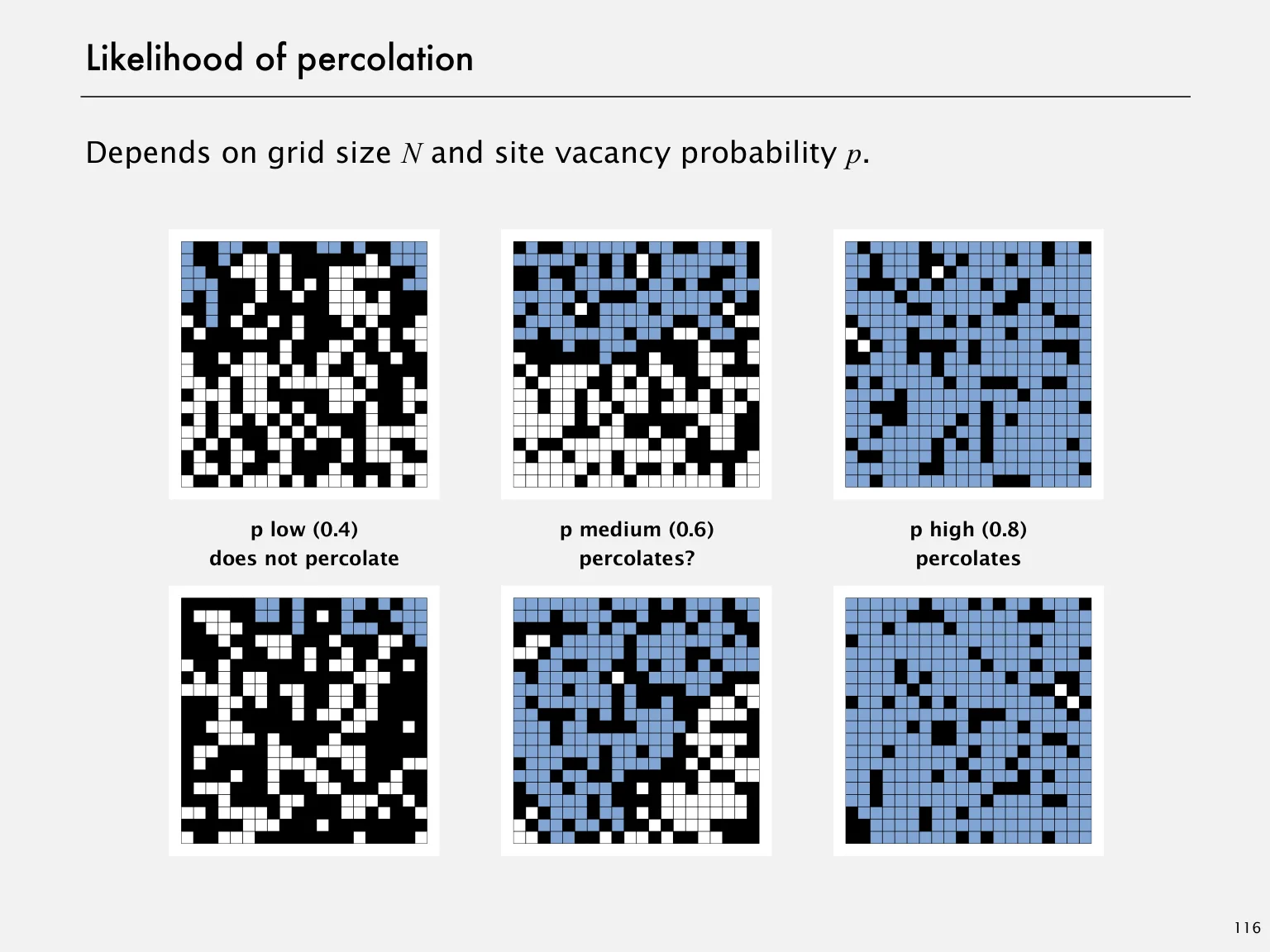
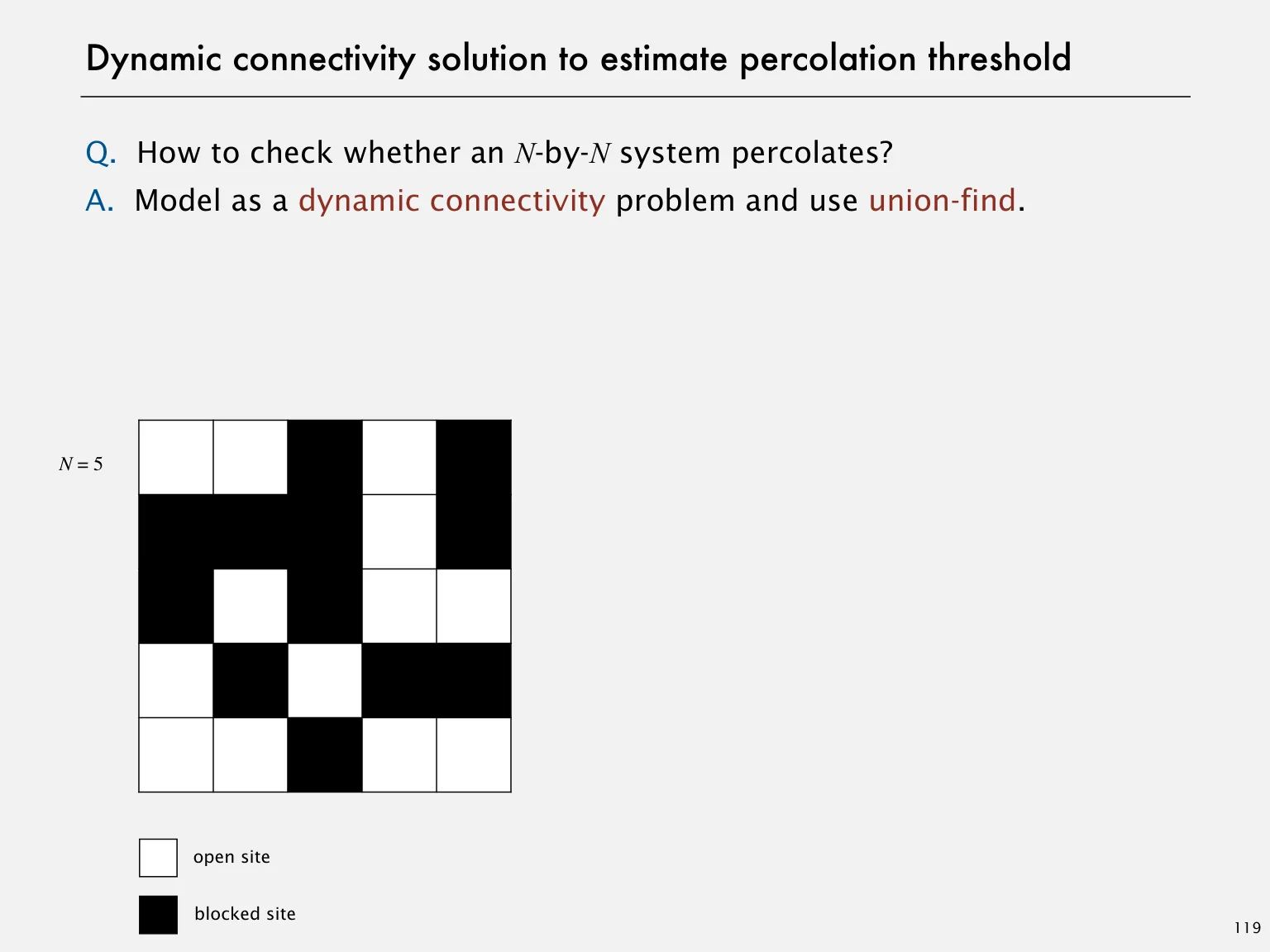
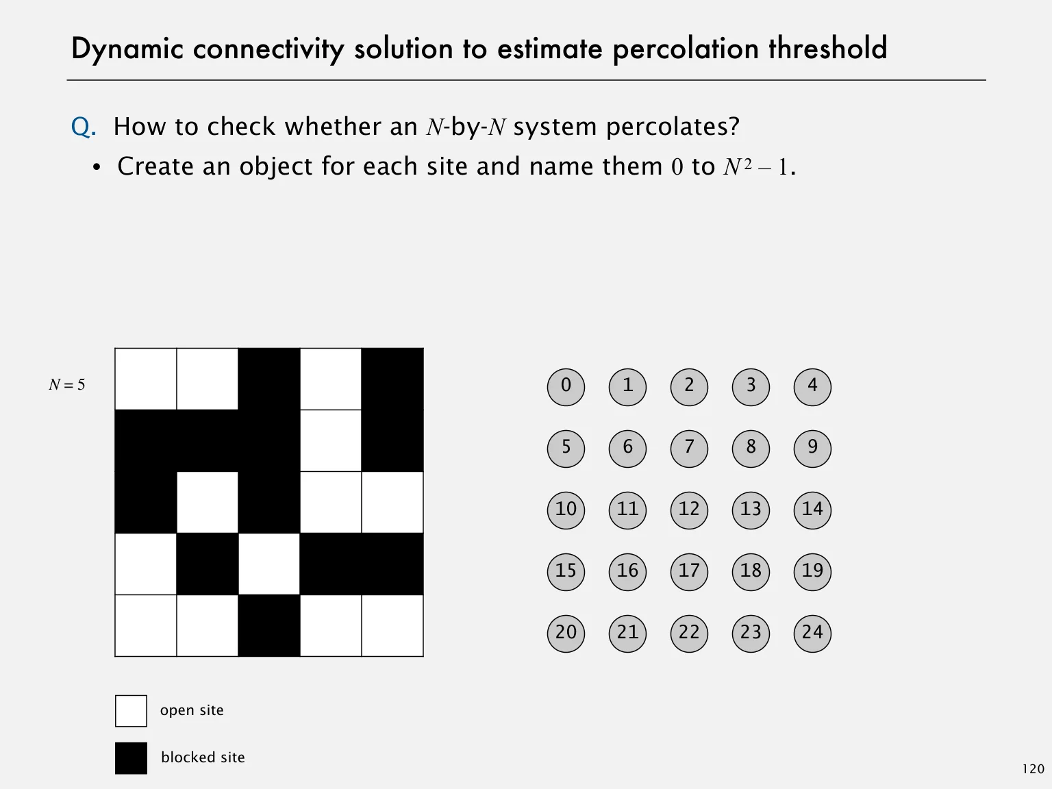
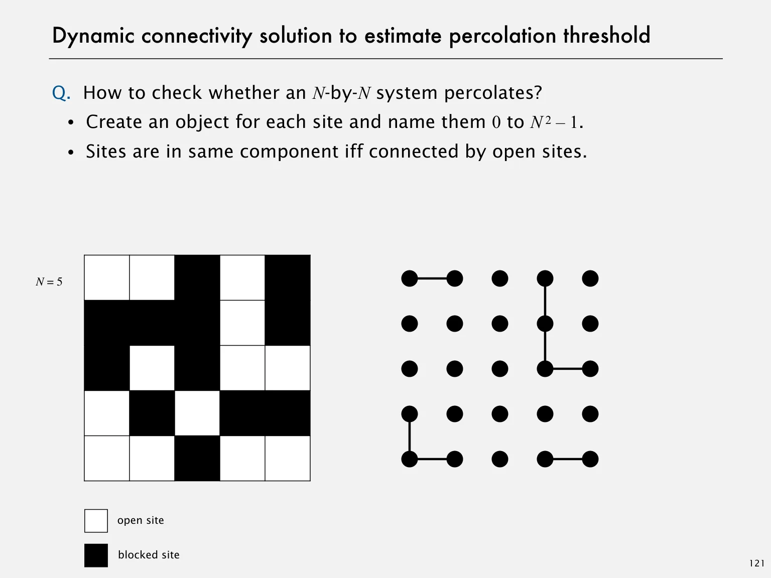
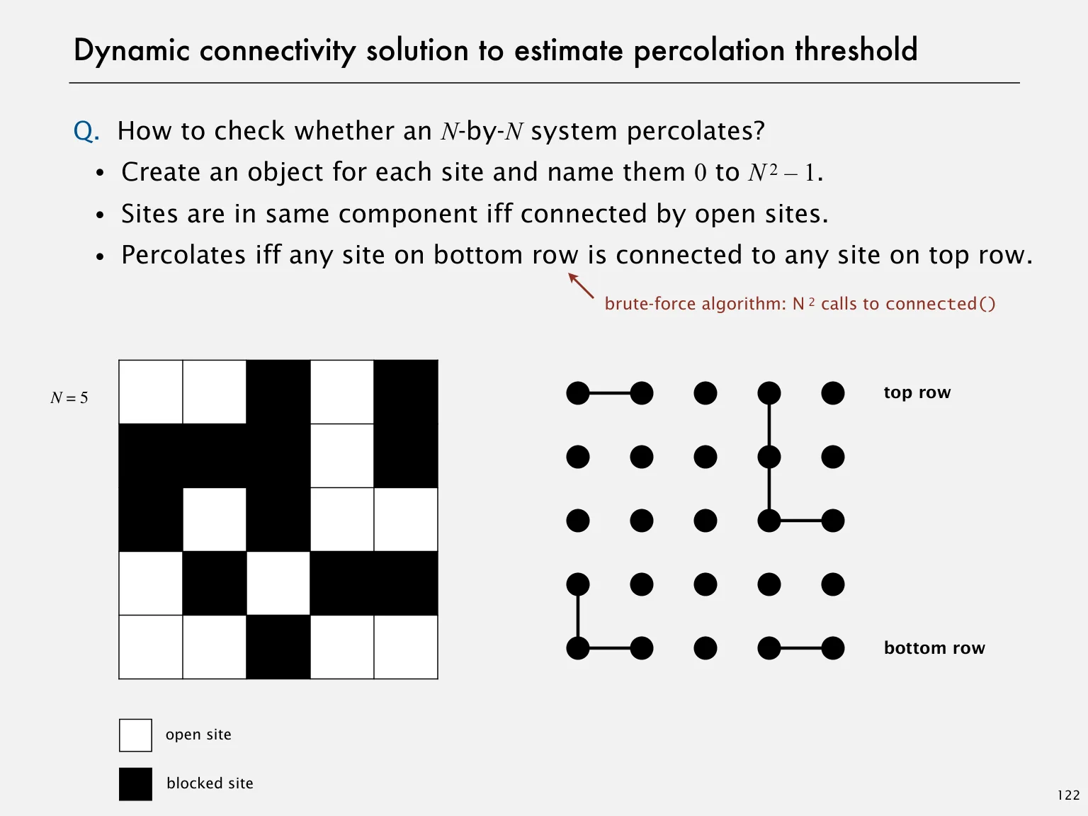
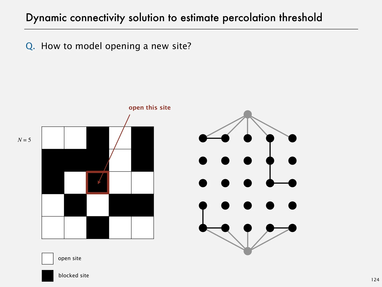
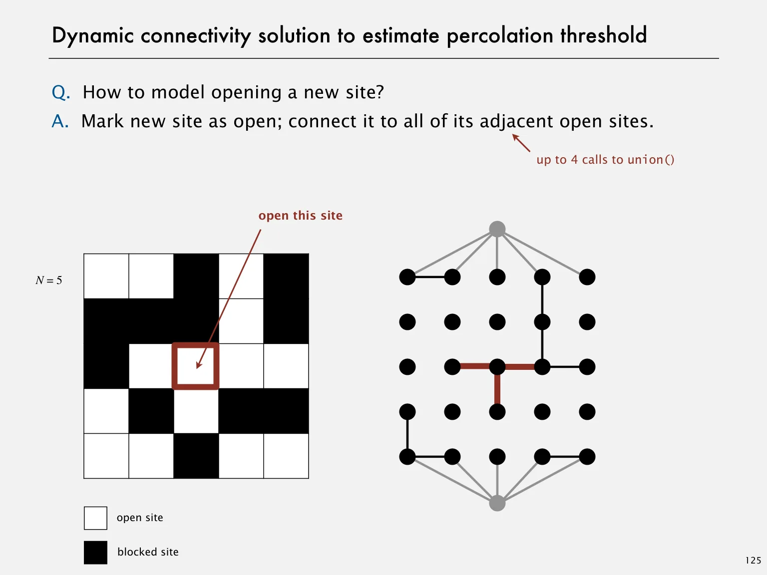
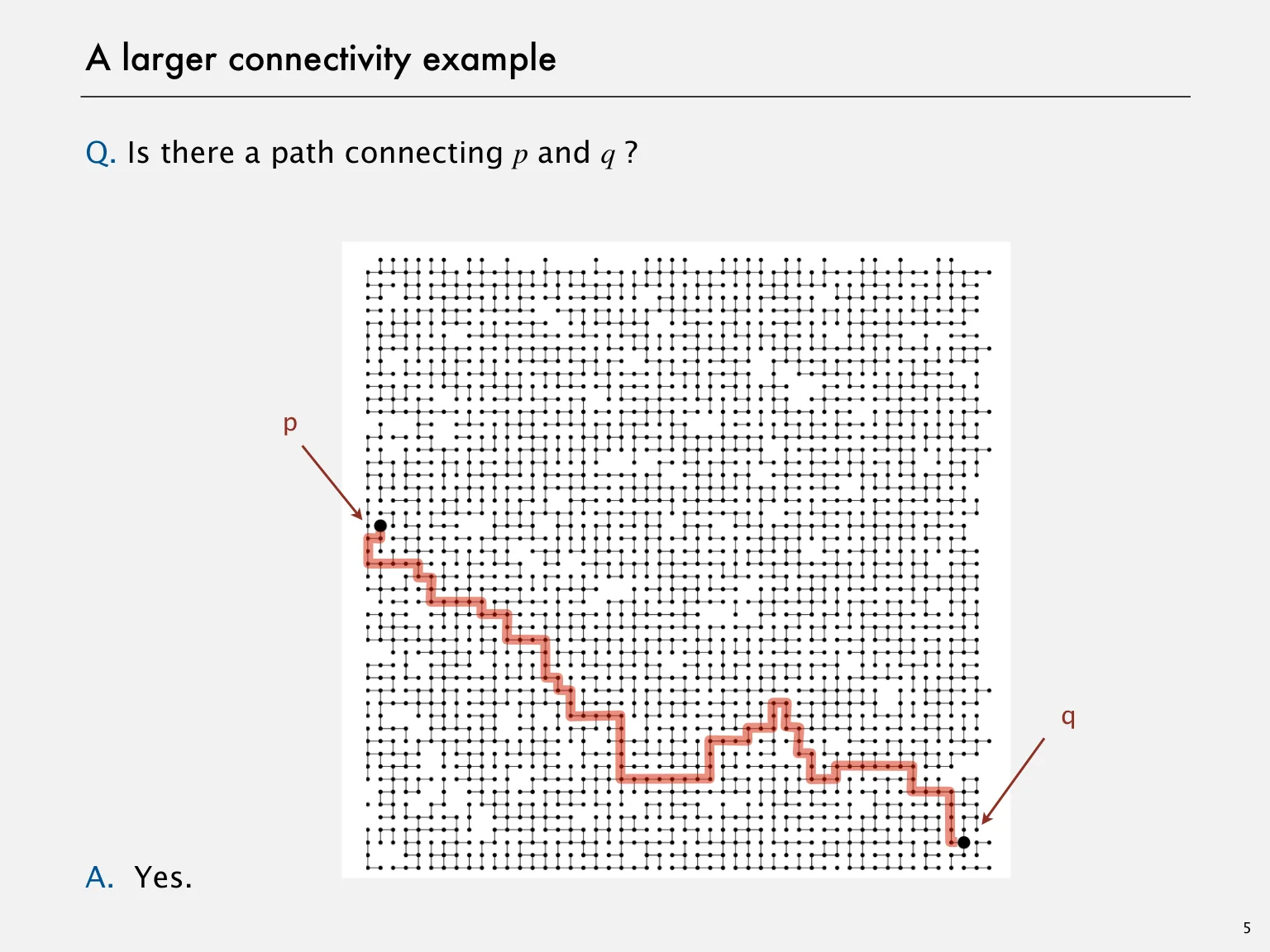
The source models an n-by-n grid of blocked or open sites. When a site opens, connect it to adjacent open sites. The system percolates when an open path connects the top row to the bottom row.
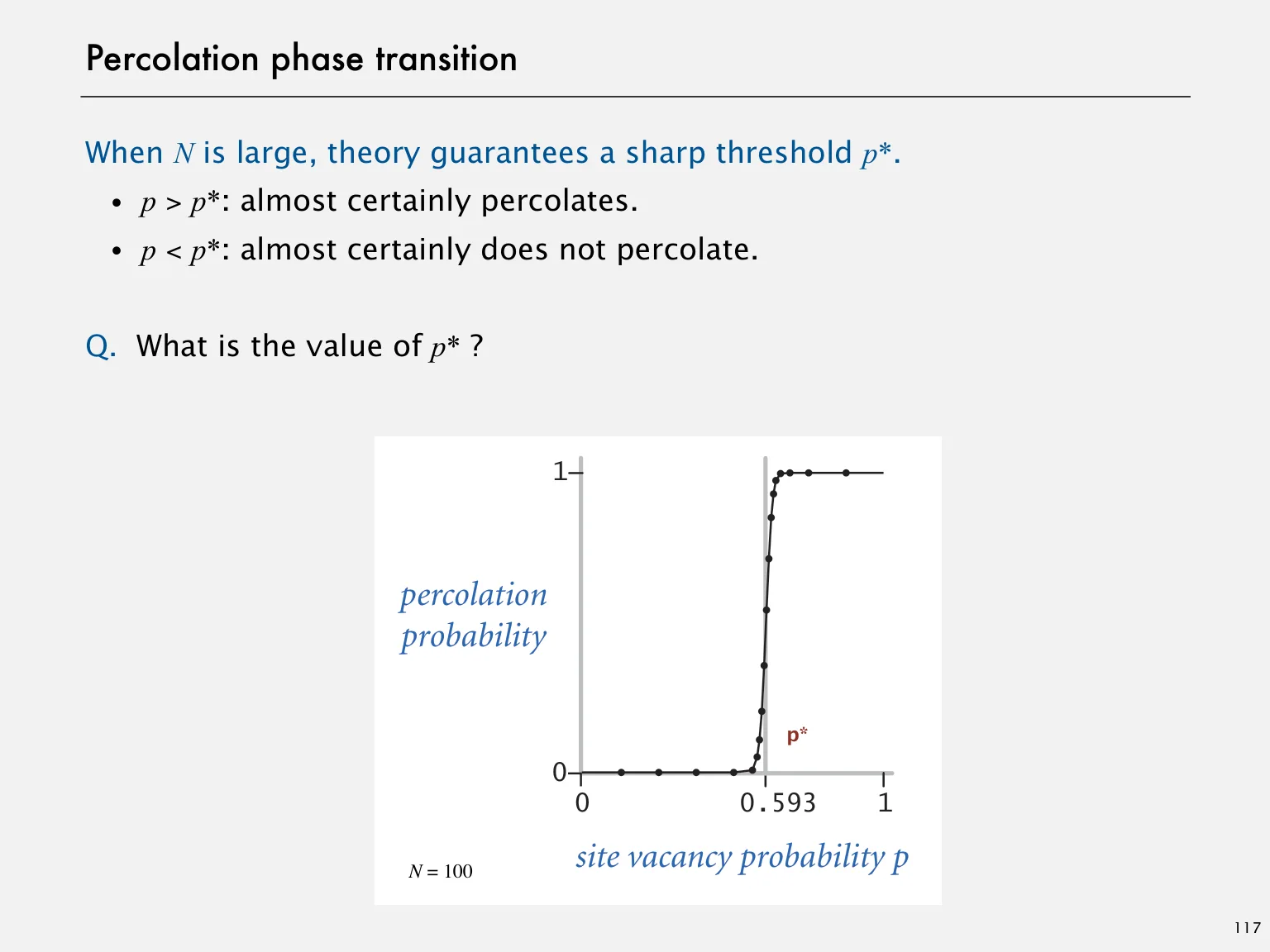
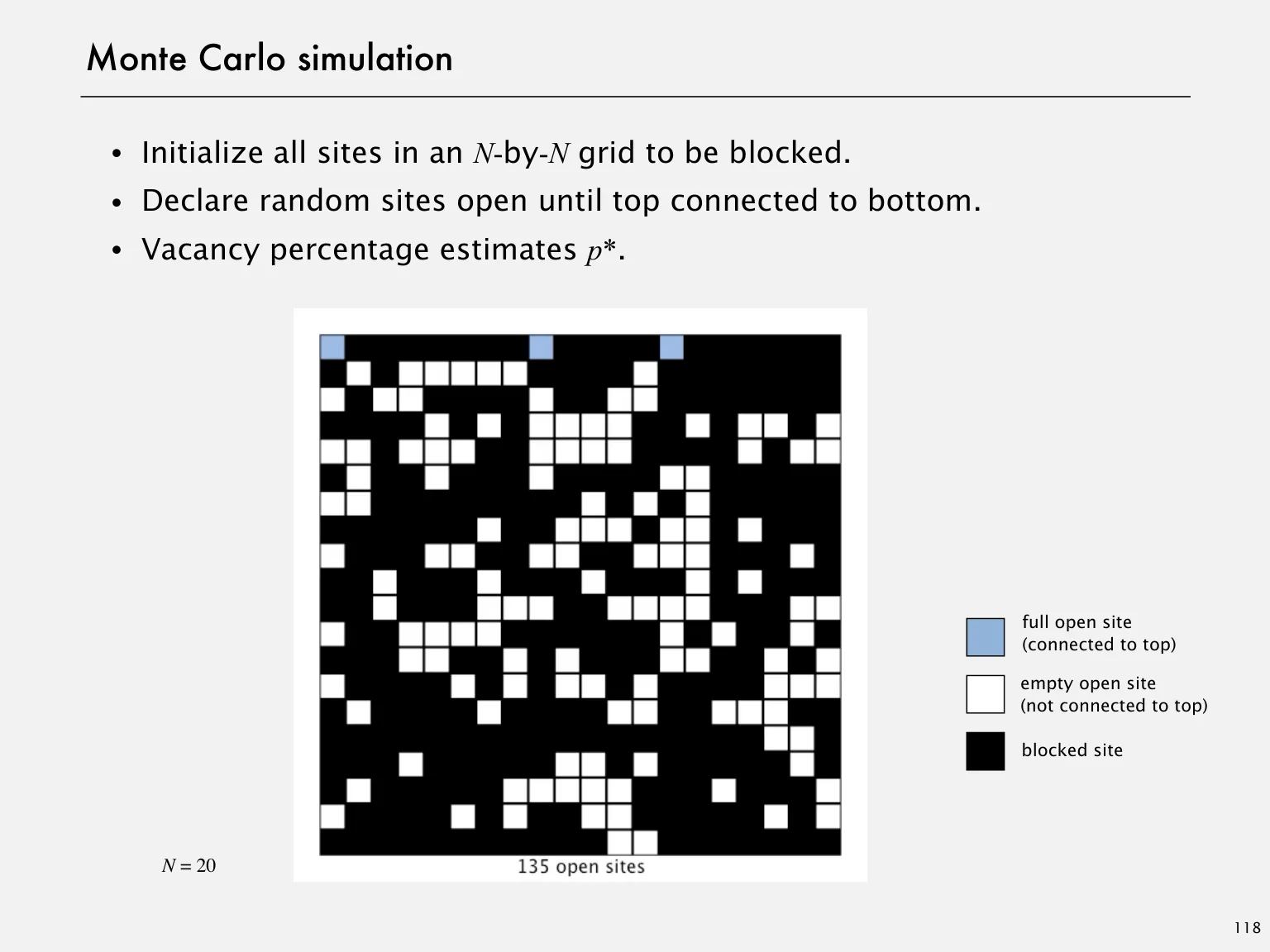
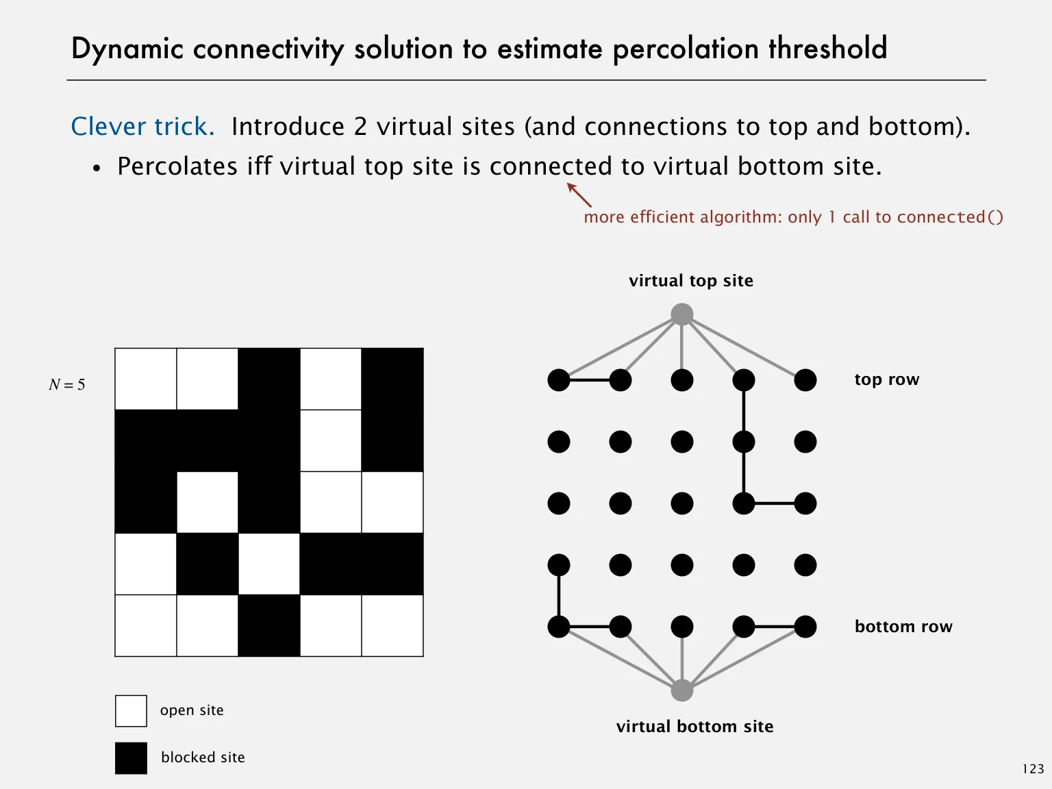
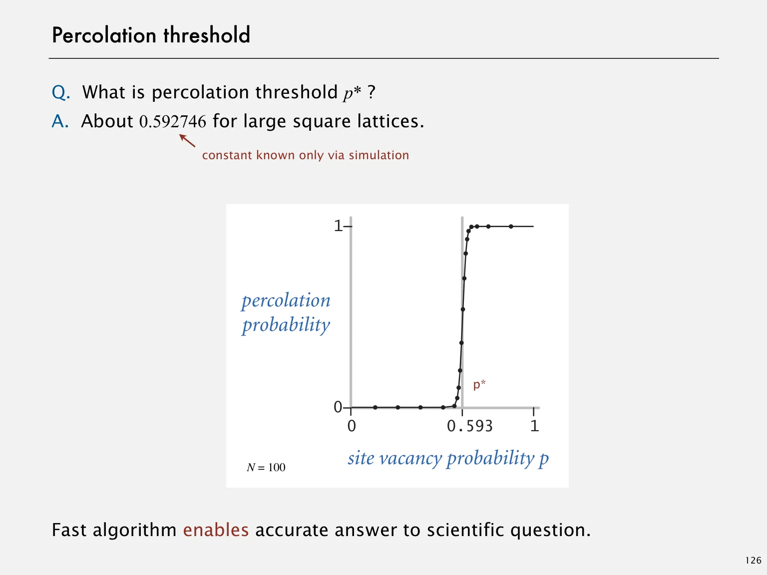
Virtual top and bottom sites reduce the percolation query to a connectivity query. Randomly opening sites until percolation occurs gives one Monte Carlo estimate of the threshold; repeat trials to study variation. The lecture’s approximate threshold is a simulation result for its specified square-lattice model.
The supplied Percolation.java actually uses recursive depth-first search to mark open sites reachable from the top, rather than the slides’ union–find implementation. It computes a fresh reachability matrix for the query. These are two different solutions to the same connectivity question.
As a supplementary caution for the virtual-site approach, one union–find structure using both virtual sites can produce backwash when testing fullness after percolation. Distinguish a percolation test from a test of whether an individual site is connected to the top.
Choosing an implementation
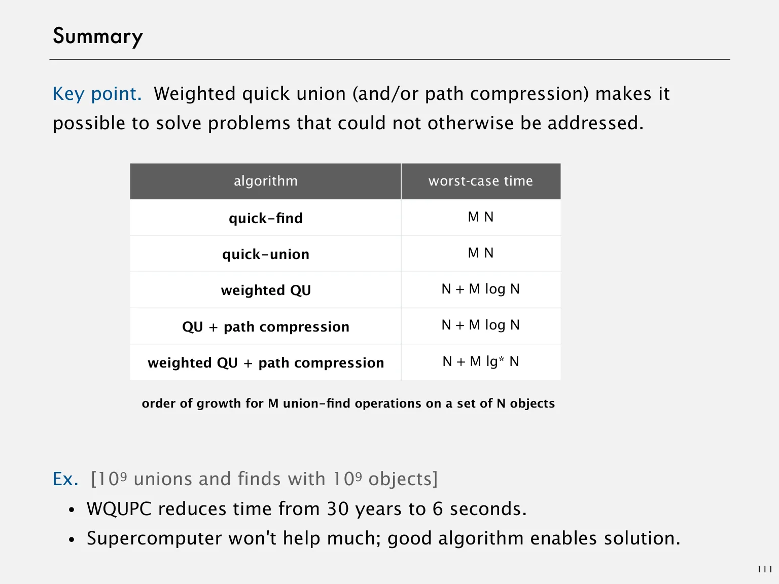
Quick-find makes lookup cheap by making updates expensive. Quick-union delays work but can grow deep trees. Weighting controls tree height; path compression speeds later operations. Always name the variant when quoting a bound.
Original implementations
Read the complete original code and its documentation. Core algorithm pages add a walkthrough, complexity discussion and a worked example.
Supplementary practice. Try each question before opening the answer.
Why must weighted union compare sizes at roots?
Only a root’s stored size represents the entire component. A non-root’s size may be stale after its tree is attached elsewhere.
Can union–find directly support deleting an arbitrary connection?
The standard structures here support merges but not efficient arbitrary splitting. Removing an edge may require a different dynamic connectivity approach.
Does amortized O(α(n)) mean every operation takes constant time?
No. It is a bound on aggregate cost over a sequence, expressed using a slowly growing function.
Original course material
Complete lecture source
Every source page is preserved below. Open a page to read its text and inspect the original diagram, formula or example. Expanded explanations above are supplementary.
Page 01 · ROBERT SEDGEWICK | KEVIN WAYNE AlgorithmsOriginal page 1 · Open the image for full detail.
ROBERT SEDGEWICK | KEVIN WAYNE Algorithms
1.5 UNION-FIND
‣ dynamic connectivity
‣ quick find
‣ quick unionAlgorithmsF O U R T H E D I T I O N
‣ improvements
‣ applications
ROBERT SEDGEWICK | KEVIN WAYNE
http://algs4.cs.princeton.edu
Page 02 · Subtext of today’s lecture (and this course)Original page 2 · Open the image for full detail.
Subtext of today’s lecture (and this course)
Steps to developing a usable algorithm.
the problem.・Model
an algorithm to solve it.・Find
enough? Fits in memory?・Fast
not, figure out why not.・If
a way to address the problem.・Find
until satisfied.・Iterate
The scientific method.
Mathematical analysis.
2
Page 03 · 1.5 UNION-FINDOriginal page 3 · Open the image for full detail.
1.5 UNION-FIND
‣ dynamic connectivity
‣ quick find
‣ quick unionAlgorithms
‣ improvements
‣ applications
ROBERT SEDGEWICK | KEVIN WAYNE
http://algs4.cs.princeton.edu
Page 04 · Dynamic connectivity problemOriginal page 4 · Open the image for full detail.
Dynamic connectivity problem
Given a set of N objects, support two operation:
two objects.・Connect
there a path connecting the two objects?・Is
connect 4 and 3
connect 3 and 8
0 1 2 3 4
connect 6 and 5
connect 9 and 4
connect 2 and 1
5 6 7 8 9
are 0 and 7 connected? 𐄂
are 8 and 9 connected? ✔
connect 5 and 0
connect 7 and 2
connect 6 and 1
connect 1 and 0
are 0 and 7 connected? ✔
4
Page 05 · A larger connectivity exampleOriginal page 5 · Open the image for full detail.
A larger connectivity example
Q. Is there a path connecting p and q ?
p
q
A. Yes.
5
Page 06 · Modeling the objectsOriginal page 6 · Open the image for full detail.
Modeling the objects
Applications involve manipulating objects of all types.
in a digital photo.・Pixels
in a network.・Computers
in a social network.・Friends
in a computer chip.・Transistors
in a mathematical set.・Elements
names in a Fortran program.・Variable
sites in a composite system.・Metallic
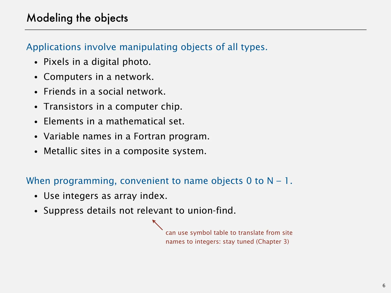
When programming, convenient to name objects 0 to N – 1.
integers as array index.・Use
details not relevant to union-find.・Suppress
can use symbol table to translate from site
names to integers: stay tuned (Chapter 3)
6
Page 07 · Modeling the connectionsOriginal page 7 · Open the image for full detail.
Modeling the connections
We assume "is connected to" is an equivalence relation:
p is connected to p.・Reflexive:
if p is connected to q, then q is connected to p.・Symmetric:
if p is connected to q and q is connected to r,・Transitive:
then p is connected to r.
Connected component. Maximal set of objects that are mutually connected.
0 1 2 3
4 5 6 7
{ 0 } { 1 4 5 } { 2 3 6 7 }
3 connected components
7
Page 08 · Implementing the operationsOriginal page 8 · Open the image for full detail.
Implementing the operations
Find. In which component is object p ?
Connected. Are objects p and q in the same component?
Union. Replace components containing objects p and q with their union.
0 1 2 3 0 1 2 3
union(2, 5)
4 5 6 7 4 5 6 7
{ 0 } { 1 4 5 } { 2 3 6 7 } { 0 } { 1 2 3 4 5 6 7 }
3 connected components 2 connected components
8
Page 09 · Union-find data type (API)Original page 9 · Open the image for full detail.
Union-find data type (API)
Goal. Design efficient data structure for union-find.
of objects N can be huge.・Number
of operations M can be huge.・Number
and find operations may be intermixed.・Union
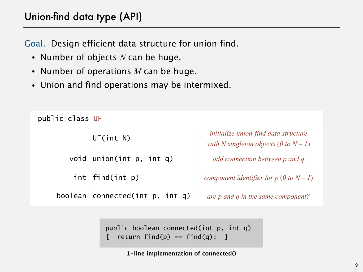
public class UF
initialize union-find data structure
UF(int N)
with N singleton objects (0 to N – 1)
void union(int p, int q) add connection between p and q
int find(int p) component identifier for p (0 to N – 1)
boolean connected(int p, int q) are p and q in the same component?
public boolean connected(int p, int q)
{ return find(p) == find(q); }
1-line implementation of connected()
9
Page 10 · Dynamic-connectivity clientOriginal page 10 · Open the image for full detail.
Dynamic-connectivity client
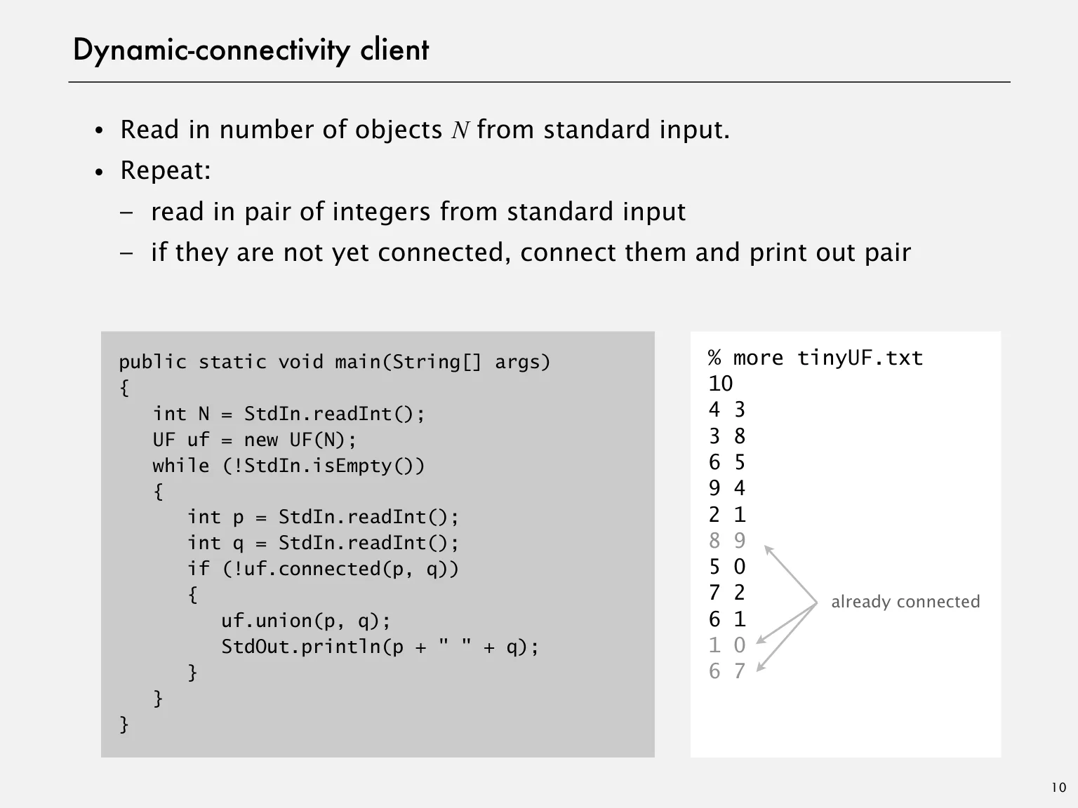
in number of objects N from standard input.・Read
・Repeat:
– read in pair of integers from standard input
– if they are not yet connected, connect them and print out pair
% more tinyUF.txt public static void main(String[] args)
{ 10
int N = StdIn.readInt(); 4 3
UF uf = new UF(N); 3 8
while (!StdIn.isEmpty()) 6 5
{ 9 4
int p = StdIn.readInt(); 2 1
int q = StdIn.readInt(); 8 9
if (!uf.connected(p, q)) 5 0
{ 7 2 already connected
uf.union(p, q); 6 1
StdOut.println(p + " " + q); 1 0
} 6 7
}
}
10
Page 11 · 1.5 UNION-FINDOriginal page 11 · Open the image for full detail.
1.5 UNION-FIND
‣ dynamic connectivity
‣ quick find
‣ quick unionAlgorithms
‣ improvements
‣ applications
ROBERT SEDGEWICK | KEVIN WAYNE
http://algs4.cs.princeton.edu
Page 12 · Quick-find [eager approach]Original page 12 · Open the image for full detail.
Quick-find [eager approach]
Data structure.
if and only if
array id[] of length N.・Integer
id[p] is the id of the component containing p.・Interpretation:
0 1 2 3 4 5 6 7 8 9
0, 5 and 6 are connected
id[] 0 1 1 8 8 0 0 1 8 8 1, 2, and 7 are connected
3, 4, 8, and 9 are connected
0 1 2 3 4
5 6 7 8 9
12
Page 13 · Quick-find [eager approach]Original page 13 · Open the image for full detail.
Quick-find [eager approach]
Data structure.
array id[] of length N.・Integer
id[p] is the id of the component containing p.・Interpretation:
0 1 2 3 4 5 6 7 8 9
id[] 0 1 1 8 8 0 0 1 8 8
Find. What is the id of p? id[6] = 0; id[1] = 1
6 and 1 are not connected
Connected. Do p and q have the same id?
Union. To merge components containing p and q, change all entries
whose id equals id[p] to id[q].
0 1 2 3 4 5 6 7 8 9
id[] 1 1 1 8 8 1 1 1 8 8 after union of 6 and 1
problem: many values can change
13
Page 14 · Quick-find demoOriginal page 14 · Open the image for full detail.
Page 26 · Quick-find: Java implementationOriginal page 26 · Open the image for full detail.
Quick-find: Java implementation
public class QuickFindUF
{
private int[] id;
public QuickFindUF(int N)
{
id = new int[N];
set id of each object to itself
for (int i = 0; i < N; i++) (N array accesses)
id[i] = i;
}
return the id of p
public boolean find(int p) (1 array access)
{ return id[p]; }
public void union(int p, int q)
{
int pid = id[p];
int qid = id[q];
change all entries with id[p] to id[q]
for (int i = 0; i < id.length; i++) (at most 2N + 2 array accesses)
if (id[i] == pid) id[i] = qid;
}
}
26
Page 27 · Quick-find is too slowOriginal page 27 · Open the image for full detail.
Quick-find is too slow
Cost model. Number of array accesses (for read or write).
algorithm initialize union find connected
quick-find N N 1 1
order of growth of number of array accesses
quadratic
Union is too expensive. It takes N 2 array accesses to process
a sequence of N union operations on N objects.
27
Page 28 · Quadratic algorithms do not scaleOriginal page 28 · Open the image for full detail.
Quadratic algorithms do not scale
Rough standard (for now).
a truism (roughly)
operations per second. since 1950!・109
words of main memory.・109
all words in approximately 1 second.・Touch
Ex. Huge problem for quick-find.
union commands on 109 objects.・109
takes more than 1018 operations.・Quick-find
years of computer time! time・30+
quadratic
64T
Quadratic algorithms don't scale with technology.
computer may be 10x as fast.・New
32T has 10x as much memory ⇒・But,
want to solve a problem that is 10x as big.
16T
linearithmic
quadratic algorithm, takes 10x as long!・With 8T
linear
size 1K 2K 4K 8K
28
Page 29 · 1.5 UNION-FINDOriginal page 29 · Open the image for full detail.
1.5 UNION-FIND
‣ dynamic connectivity
‣ quick find
‣ quick unionAlgorithms
‣ improvements
‣ applications
ROBERT SEDGEWICK | KEVIN WAYNE
http://algs4.cs.princeton.edu
Page 30 · Quick-union [lazy approach]Original page 30 · Open the image for full detail.
Quick-union [lazy approach]
Data structure.
array id[] of length N.・Integer keep going until it doesn’t change
id[i] is parent of i. (algorithm ensures no cycles)・Interpretation:
of i is id[id[id[...id[i]...]]].・Root
0 1 9 6 7 8
0 1 2 3 4 5 6 7 8 9
2 4 5
id[] 0 1 9 4 9 6 6 7 8 9
3
parent of 3 is 4
root of 3 is 9
30
Page 31 · Quick-union [lazy approach]Original page 31 · Open the image for full detail.
Quick-union [lazy approach]
Data structure.
array id[] of length N.・Integer
id[i] is parent of i.・Interpretation:
of i is id[id[id[...id[i]...]]].・Root
0 1 9 6 7 8
0 1 2 3 4 5 6 7 8 9
2 4 5 q
id[] 0 1 9 4 9 6 6 7 8 9
p 3
Find. What is the root of p? root of 3 is 9
root of 5 is 6
Connected. Do p and q have the same root? 3 and 5 are not connected
Union. To merge components containing p and q, 0 1 6 7 8
set the id of p's root to the id of q's root.
9
5 q
0 1 2 3 4 5 6 7 8 9
id[] 0 1 9 4 9 6 6 7 8 6 2 4
p 3
only one value changes 31
Page 32 · Quick-union demoOriginal page 32 · Open the image for full detail.
Page 62 · Quick-union: Java implementationOriginal page 62 · Open the image for full detail.
Quick-union: Java implementation
public class QuickUnionUF
{
private int[] id;
public QuickUnionUF(int N)
{
set id of each object to itself id = new int[N];
for (int i = 0; i < N; i++) id[i] = i; (N array accesses)
}
public int find(int i)
{
while (i != id[i]) i = id[i]; chase parent pointers until reach root
return i; (depth of i array accesses)
}
public void union(int p, int q)
{
int i = find(p); change root of p to point to root of q
int j = find(q); (depth of p and q array accesses)
id[i] = j;
}
}
62
Page 63 · Quick-union is also too slowOriginal page 63 · Open the image for full detail.
Quick-union is also too slow
Cost model. Number of array accesses (for read or write).
algorithm initialize union find connected
quick-find N N 1 1
quick-union N N † N N worst case
† includes cost of finding roots
Quick-find defect.
too expensive (N array accesses).・Union
are flat, but too expensive to keep them flat.・Trees
Quick-union defect.
can get tall.・Trees
too expensive (could be N array accesses).・Find/connected
63
Page 64 · 1.5 UNION-FINDOriginal page 64 · Open the image for full detail.
1.5 UNION-FIND
‣ dynamic connectivity
‣ quick find
‣ quick unionAlgorithms
‣ improvements
‣ applications
ROBERT SEDGEWICK | KEVIN WAYNE
http://algs4.cs.princeton.edu
Page 65 · Improvement 1: weightingOriginal page 65 · Open the image for full detail.
Improvement 1: weighting
Weighted quick-union.
quick-union to avoid tall trees.・Modify
track of size of each tree (number of objects).・Keep
by linking root of smaller tree to root of larger tree.・Balance
reasonable alternatives:
quick-union q union by height or "rank" p
smaller
p tree q
smaller larger
tree tree might put the
larger larger tree lower
tree
weighted
always chooses the p p
better alternative
q q
smaller smaller larger larger
tree tree tree tree
65
Page 66 · Weighted quick-union demoOriginal page 66 · Open the image for full detail.
Page 95 · Quick-union and weighted quick-union exampleOriginal page 95 · Open the image for full detail.
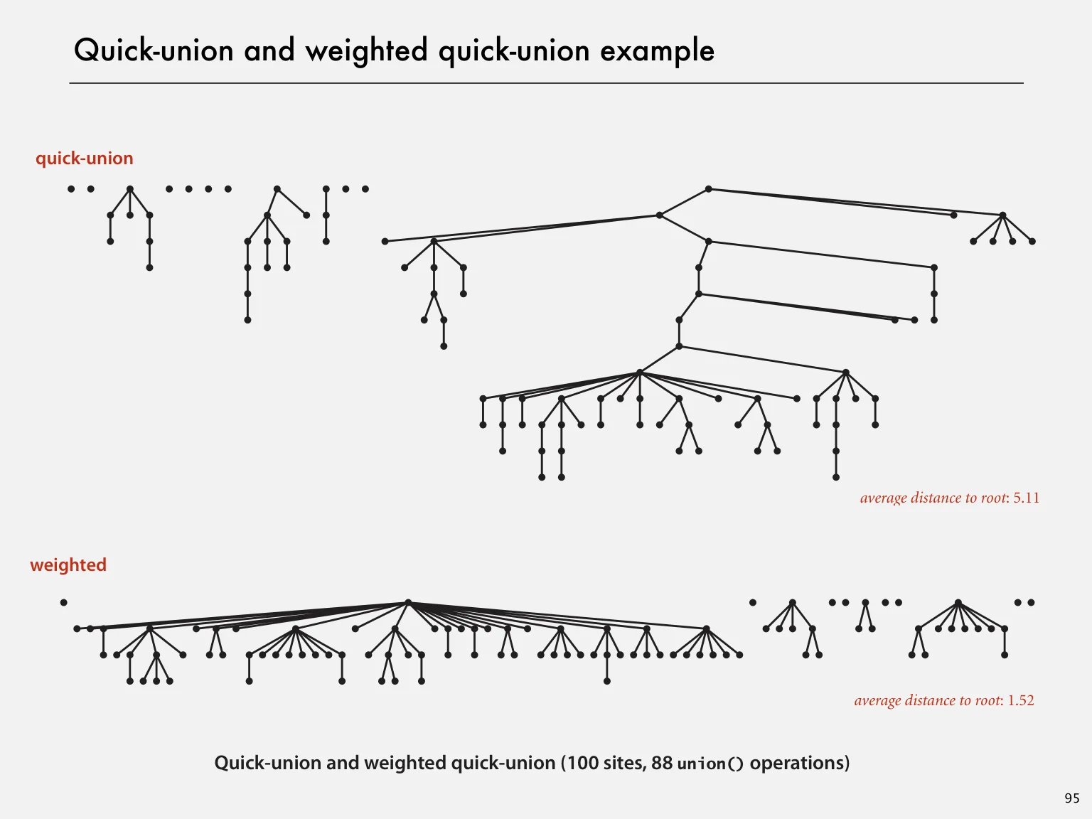
Quick-union and weighted quick-union example
quick-union
average distance to root: 5.11
weighted
average distance to root: 1.52
Quick-union and weighted quick-union (100 sites, 88 union() operations)
95
Page 96 · Weighted quick-union: Java implementationOriginal page 96 · Open the image for full detail.
Weighted quick-union: Java implementation
Data structure. Same as quick-union, but maintain extra array sz[i]
to count number of objects in the tree rooted at i.
Find/connected. Identical to quick-union.
Union. Modify quick-union to:
root of smaller tree to root of larger tree.・Link
the sz[] array.・Update
int i = find(p);
int j = find(q);
if (i == j) return;
if (sz[i] < sz[j]) { id[i] = j; sz[j] += sz[i]; }
else { id[j] = i; sz[i] += sz[j]; }
96
Page 97 · Weighted quick-union analysisOriginal page 97 · Open the image for full detail.
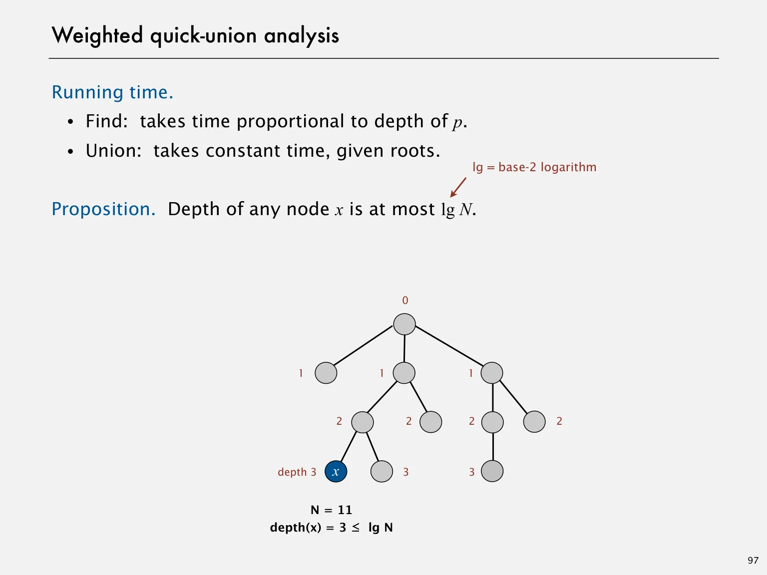
Weighted quick-union analysis
Running time.
takes time proportional to depth of p.・Find:
takes constant time, given roots.・Union:
lg = base-2 logarithm
Proposition. Depth of any node x is at most lg N.
0
1 1 1
2 2 2 2
depth 3 x 3 3
N = 11
depth(x) = 3 ≤ lg N
97
Page 98 · Weighted quick-union analysisOriginal page 98 · Open the image for full detail.
Weighted quick-union analysis
Running time.
takes time proportional to depth of p.・Find:
takes constant time, given roots.・Union:
lg = base-2 logarithm
Proposition. Depth of any node x is at most lg N.
Pf. What causes the depth of object x to increase?
Increases by 1 when tree T1 containing x is merged into another tree T2.
size of the tree containing x at least doubles since | T 2 | ≥ | T 1 |.・The
of tree containing x can double at most lg N times. Why?・Size
1
2
4
T2 8 lg N
16 T1
⋮
x
N
98
Page 99 · Weighted quick-union analysisOriginal page 99 · Open the image for full detail.
Weighted quick-union analysis
99
Page 100 · Weighted quick-union analysisOriginal page 100 · Open the image for full detail.
Weighted quick-union analysis
100
Page 101 · Weighted quick-union analysisOriginal page 101 · Open the image for full detail.
Weighted quick-union analysis
101
Page 102 · Weighted quick-union analysisOriginal page 102 · Open the image for full detail.
Weighted quick-union analysis
102
Page 103 · Weighted quick-union analysisOriginal page 103 · Open the image for full detail.
Weighted quick-union analysis
Running time.
takes time proportional to depth of p.・Find:
takes constant time, given roots.・Union:
Proposition. Depth of any node x is at most lg N.
algorithm initialize union find connected
quick-find N N 1 1
quick-union N N † N N
weighted QU N lg N † lg N lg N
† includes cost of finding roots
Q. Stop at guaranteed acceptable performance?
A. No, easy to improve further.
103
Page 104 · Improvement 2: path compressionOriginal page 104 · Open the image for full detail.
Improvement 2: path compression
Quick union with path compression. Just after computing the root of p,
set the id[] of each examined node to point to that root.
0 root
1 2
3 4 5
6 7
p
8 x 9
10 11 12
104
Page 105 · Improvement 2: path compressionOriginal page 105 · Open the image for full detail.
Improvement 2: path compression
Quick union with path compression. Just after computing the root of p,
set the id[] of each examined node to point to that root.
0 root
p
9 1 2
11 12 3 4 5
x 6 7
8
10
105
Page 106 · Improvement 2: path compressionOriginal page 106 · Open the image for full detail.
Improvement 2: path compression
Quick union with path compression. Just after computing the root of p,
set the id[] of each examined node to point to that root.
0 root
p
9 6 1 2
11 12 8 x 3 4 5
10 7
106
Page 107 · Improvement 2: path compressionOriginal page 107 · Open the image for full detail.
Improvement 2: path compression
Quick union with path compression. Just after computing the root of p,
set the id[] of each examined node to point to that root.
0 root
p
9 6 3 x 1 2
11 12 8 7 4 5
10
107
Page 108 · Improvement 2: path compressionOriginal page 108 · Open the image for full detail.
Improvement 2: path compression
Quick union with path compression. Just after computing the root of p,
set the id[] of each examined node to point to that root.
x
0 root
p
9 6 3 1 2
11 12 8 7 4 5
10
Bottom line. Now, find() has the side effect of compressing the tree.
108
Page 109 · Path compression: Java implementationOriginal page 109 · Open the image for full detail.
Path compression: Java implementation
Two-pass implementation: add second loop to find() to set the id[]
of each examined node to the root.
Simpler one-pass variant (path halving): Make every other node in path
point to its grandparent.
public int find(int i)
{
while (i != id[i])
{
id[i] = id[id[i]]; only one extra line of code !
i = id[i];
}
return i;
}
In practice. No reason not to! Keeps tree almost completely flat.
109
Page 110 · Weighted quick-union with path compression: amortized analysisOriginal page 110 · Open the image for full detail.
Weighted quick-union with path compression: amortized analysis
Proposition. [Hopcroft-Ulman, Tarjan] Starting from an N lg* N
empty data structure, any sequence of M union-find ops 1 0
on N objects makes ≤ c ( N + M lg* N ) array accesses. 2 1
can be improved to N + M α(M, N).・Analysis 4 2
algorithm with fascinating mathematics.・Simple 16 3
65536 4
265536 5
iterated lg function
Linear-time algorithm for M union-find ops on N objects?
within constant factor of reading in the data.・Cost
theory, WQUPC is not quite linear.・In
practice, WQUPC is linear.・In
Amazing fact. [Fredman-Saks] No linear-time algorithm exists.
in "cell-probe" model of computation
110
Page 111 · SummaryOriginal page 111 · Open the image for full detail.
Summary
Key point. Weighted quick union (and/or path compression) makes it
possible to solve problems that could not otherwise be addressed.
algorithm worst-case time
quick-find M N
quick-union M N
weighted QU N + M log N
QU + path compression N + M log N
weighted QU + path compression N + M lg* N
order of growth for M union-find operations on a set of N objects
Ex. [109 unions and finds with 109 objects]
reduces time from 30 years to 6 seconds.・WQUPC
won't help much; good algorithm enables solution.・Supercomputer
111
Page 112 · 1.5 UNION-FINDOriginal page 112 · Open the image for full detail.
1.5 UNION-FIND
‣ dynamic connectivity
‣ quick find
‣ quick unionAlgorithms
‣ improvements
‣ applications
ROBERT SEDGEWICK | KEVIN WAYNE
http://algs4.cs.princeton.edu
Page 113 · Union-find applicationsOriginal page 113 · Open the image for full detail.
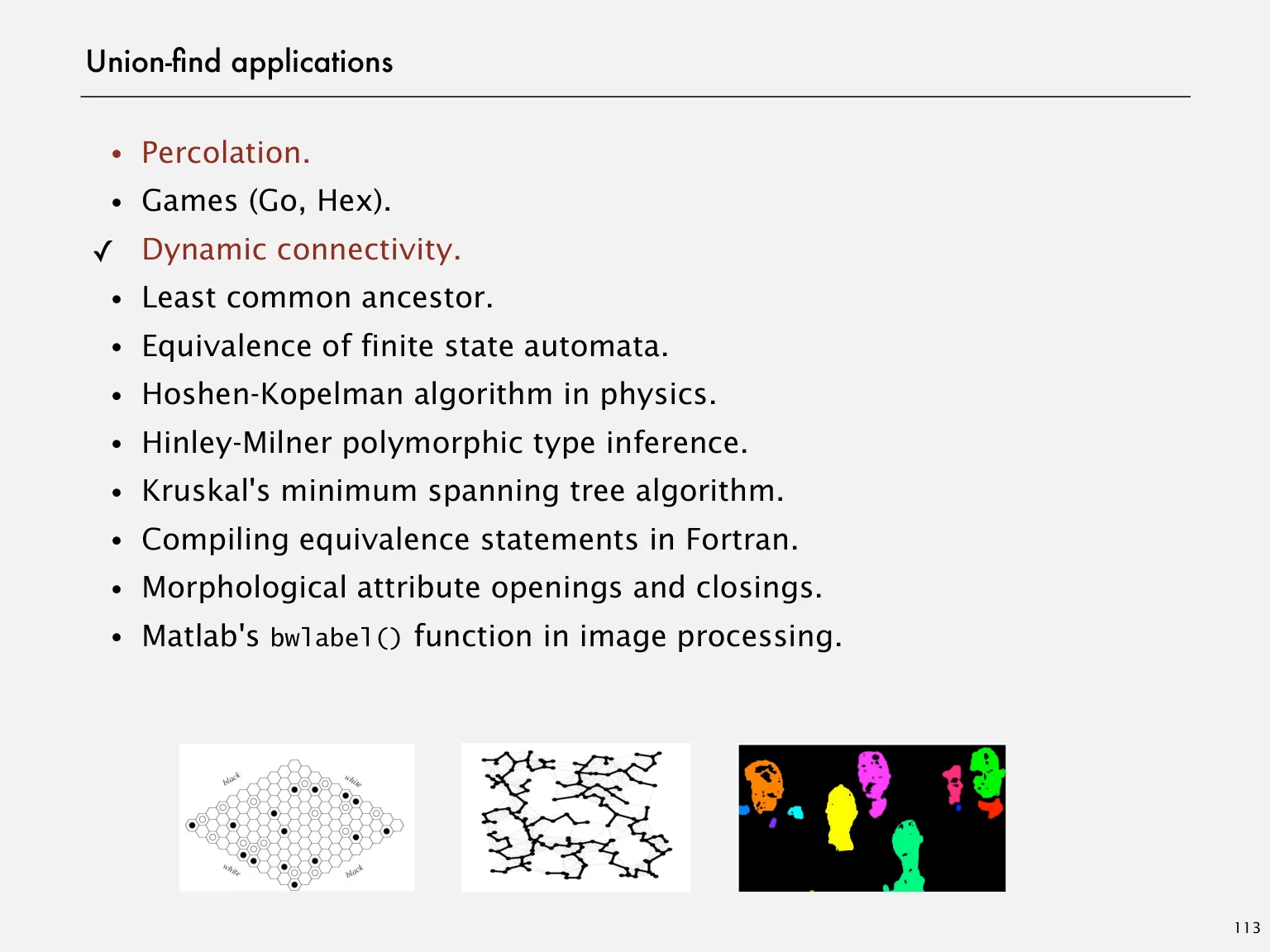
Union-find applications
・Percolation.
(Go, Hex).・Games
✓ Dynamic connectivity.
common ancestor.・Least
of finite state automata.・Equivalence
algorithm in physics.・Hoshen-Kopelman
polymorphic type inference.・Hinley-Milner
minimum spanning tree algorithm.・Kruskal's
equivalence statements in Fortran.・Compiling
attribute openings and closings.・Morphological
bwlabel() function in image processing.・Matlab's
113
Page 114 · PercolationOriginal page 114 · Open the image for full detail.
Percolation
An abstract model for many physical systems:
grid of sites.・N-by-N
site is open with probability p (and blocked with probability 1 – p).・Each
percolates iff top and bottom are connected by open sites.・System
does not percolate percolates
blocked
site
open
site
open site connected to top
no open site connected to top N = 8
114
Page 115 · PercolationOriginal page 115 · Open the image for full detail.
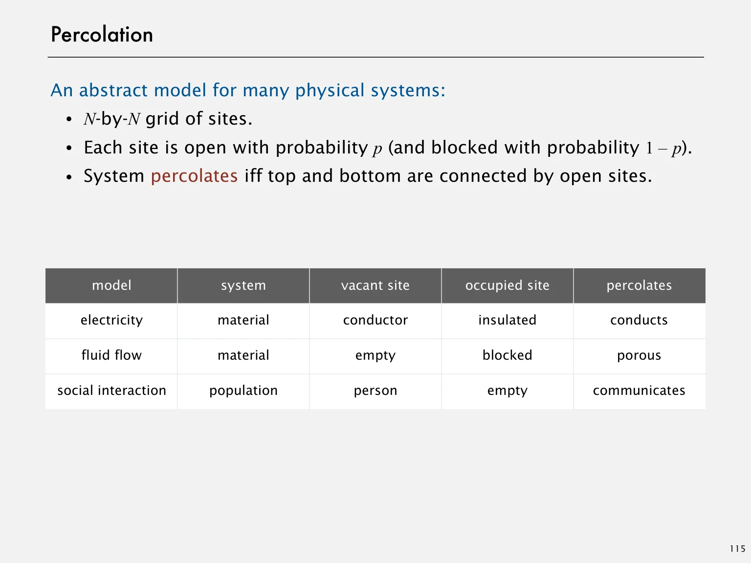
Percolation
An abstract model for many physical systems:
grid of sites.・N-by-N
site is open with probability p (and blocked with probability 1 – p).・Each
percolates iff top and bottom are connected by open sites.・System
model system vacant site occupied site percolates
electricity material conductor insulated conducts
fluid flow material empty blocked porous
social interaction population person empty communicates
115
Page 116 · Likelihood of percolationOriginal page 116 · Open the image for full detail.
Likelihood of percolation
Depends on grid size N and site vacancy probability p.
p low (0.4) p medium (0.6) p high (0.8)
does not percolate percolates? percolates
116
Page 117 · Percolation phase transitionOriginal page 117 · Open the image for full detail.
Percolation phase transition
When N is large, theory guarantees a sharp threshold p*.
> p*: almost certainly percolates.・p
< p*: almost certainly does not percolate.・p
Q. What is the value of p* ?
1
percolation
probability
p*
0
0 0.593 1
site vacancy probability p N = 100
117
Page 118 · Monte Carlo simulationOriginal page 118 · Open the image for full detail.
Monte Carlo simulation
all sites in an N-by-N grid to be blocked.・Initialize
random sites open until top connected to bottom.・Declare
percentage estimates p*.・Vacancy
full open site
(connected to top)
empty open site
(not connected to top)
blocked site
N = 20
118
Page 119 · Dynamic connectivity solution to estimate percolation thresholdOriginal page 119 · Open the image for full detail.
Dynamic connectivity solution to estimate percolation threshold
Q. How to check whether an N-by-N system percolates?
A. Model as a dynamic connectivity problem and use union-find.
N = 5
open site
blocked site
119
Page 120 · Dynamic connectivity solution to estimate percolation thresholdOriginal page 120 · Open the image for full detail.
Dynamic connectivity solution to estimate percolation threshold
Q. How to check whether an N-by-N system percolates?
an object for each site and name them 0 to N 2 – 1. ・Create
N = 5 0 1 2 3 4
5 6 7 8 9
10 11 12 13 14
15 16 17 18 19
20 21 22 23 24
open site
blocked site
120
Page 121 · Dynamic connectivity solution to estimate percolation thresholdOriginal page 121 · Open the image for full detail.
Dynamic connectivity solution to estimate percolation threshold
Q. How to check whether an N-by-N system percolates?
an object for each site and name them 0 to N 2 – 1. ・Create
are in same component iff connected by open sites. ・Sites
N = 5
open site
blocked site
121
Page 122 · Dynamic connectivity solution to estimate percolation thresholdOriginal page 122 · Open the image for full detail.
Dynamic connectivity solution to estimate percolation threshold
Q. How to check whether an N-by-N system percolates?
an object for each site and name them 0 to N 2 – 1. ・Create
are in same component iff connected by open sites. ・Sites
iff any site on bottom row is connected to any site on top row. ・Percolates
brute-force algorithm: N 2 calls to connected()
top rowN = 5
bottom row
open site
blocked site
122
Page 123 · Dynamic connectivity solution to estimate percolation thresholdOriginal page 123 · Open the image for full detail.
Dynamic connectivity solution to estimate percolation threshold
Clever trick. Introduce 2 virtual sites (and connections to top and bottom).
iff virtual top site is connected to virtual bottom site. ・Percolates
more efficient algorithm: only 1 call to connected()
virtual top site
top rowN = 5
bottom row
open site
virtual bottom site
blocked site
123
Page 124 · Dynamic connectivity solution to estimate percolation thresholdOriginal page 124 · Open the image for full detail.
Dynamic connectivity solution to estimate percolation threshold
Q. How to model opening a new site?
open this site
N = 5
open site
blocked site
124
Page 125 · Dynamic connectivity solution to estimate percolation thresholdOriginal page 125 · Open the image for full detail.
Dynamic connectivity solution to estimate percolation threshold
Q. How to model opening a new site?
A. Mark new site as open; connect it to all of its adjacent open sites.
up to 4 calls to union()
open this site
N = 5
open site
blocked site
125
Page 126 · Percolation thresholdOriginal page 126 · Open the image for full detail.
Percolation threshold
Q. What is percolation threshold p* ?
A. About 0.592746 for large square lattices.
constant known only via simulation
1
percolation
probability
p*
0
0 0.593 1
site vacancy probability p N = 100
Fast algorithm enables accurate answer to scientific question.
126
Page 127 · Subtext of today’s lecture (and this course)Original page 127 · Open the image for full detail.
Subtext of today’s lecture (and this course)
Steps to developing a usable algorithm.
the problem.・Model
an algorithm to solve it.・Find
enough? Fits in memory?・Fast
not, figure out why.・If
a way to address the problem.・Find
until satisfied.・Iterate
The scientific method.
Mathematical analysis.
127

![Original lectures/5_UnionFind.pdf, page 12: Quick-find [eager approach]](/slides/5-unionfind/12.webp)
![Original lectures/5_UnionFind.pdf, page 13: Quick-find [eager approach]](/slides/5-unionfind/13.webp)
![Original lectures/5_UnionFind.pdf, page 30: Quick-union [lazy approach]](/slides/5-unionfind/30.webp)
![Original lectures/5_UnionFind.pdf, page 31: Quick-union [lazy approach]](/slides/5-unionfind/31.webp)